Introduction to Machine Learning Talk

There was an amazing turnout at last night’s DataPhilly meetup (~200 people!). I was completely delighted by the turnout and people’s engagement level. Here are the slides of the talk I gave to set up the evening with a high-level introduction to machine learning.


Advertisement

Speaking at DataPhilly February 2016

The next DataPhilly meetup will feature a medley of machine-learning talks, including an Intro to ML from yours truly. Check out the speakers list and be sure to RSVP. Hope to see you there!

Thursday, February 18, 2016

6:00 PM to 9:00 PM

Speakers:

  • Corey Chivers
  • Randy Olson
  • Austin Rochford

Corey Chivers (Penn Medicine)

Abstract: Corey will present a brief introduction to machine learning. In his talk he will demystify what is often seen as a dark art. Corey will describe how we “teach” machines to learn patterns from examples by breaking the process into its easy-to-understand component parts. By using examples from fields as diverse as biology, health-care, astrophysics, and NBA basketball, Corey will show how data (both big and small) is used to teach machines to predict the future so we can make better decisions.

Bio: Corey Chivers is a Senior Data Scientist at Penn Medicine where he is building machine learning systems to improve patient outcomes by providing real-time predictive applications that empower clinicians to identify at risk individuals. When he’s not pouring over data, he’s likely to be found cycling around his adoptive city of Philadelphia or blogging about all things probability and data at bayesianbiologist.com.

Randy Olson (University of Pennsylvania Institute for Biomedical Informatics):

Automating data science through tree-based pipeline optimization

Abstract: Over the past decade, data science and machine learning has grown from a mysterious art form to a staple tool across a variety of fields in business, academia, and government. In this talk, I’m going to introduce the concept of tree-based pipeline optimization for automating one of the most tedious parts of machine learning — pipeline design. All of the work presented in this talk is based on the open source Tree-based Pipeline Optimization Tool (TPOT), which is available on GitHub at https://github.com/rhiever/tpot.

Bio: Randy Olson is an artificial intelligence researcher at the University of Pennsylvania Institute for Biomedical Informatics, where he develops state-of-the-art machine learning algorithms to solve biomedical problems. He regularly writes about his latest adventures in data science at RandalOlson.com/blog, and tweets about the latest data science news at http://twitter.com/randal_olson.

Austin Rochford (Monetate):

Abstract: Bayesian optimization is a technique for finding the extrema of functions which are expensive, difficult, or time-consuming to evaluate. It has many applications to optimizing the hyperparameters of machine learning models, optimizing the inputs to real-world experiments and processes, etc. This talk will introduce the Gaussian process approach to Bayesian optimization, with sample code in Python.

Bio: Austin Rochford is a Data Scientist at Monetate. He is a former mathematician who is interested in Bayesian nonparametrics, multilevel models, probabilistic programming, and efficient Bayesian computation.

A probabilistic justification to carpe diem

There’s a curious thing about unlikely independent events: no matter how rare, they’re most likely to happen right away.

Let’s get hypothetical

You’ve taken a bet that pays off if you guess the exact date of the next occurrence of a rare event (p = 0.0001 on any given day i.i.d). What day do you choose? In other words, what is the most likely day for this rare event to occur?

Setting aside for now why in the world you’ve taken such a silly sounding bet, it would seem as though a reasonable way to think about it would be to ask: what is the expected number of days until the event? That must be the best bet, right?

We can work out the expected number of days quite easily as 1/p = 10000. So using the logic of expectation, we would choose day 10000 as our bet.

Let’s simulate to see how often we would win with this strategy. We’ll simulate the outcomes by flipping a weighted coin until it comes out heads. We’ll do this 100,000 times and record how many flips it took each time.

p0001

The event occurred on day 10,000 exactly 35 times. However, if we look at a histogram of our simulation experiment, we can see that the time it took for the rare event to happen was more often short, than long. In fact, the event occurred 103 times on the very first flip (the most common Time to Event in our set)!

So from the experiment it would seem that the most likely amount of time to pass until the rare event occurs is 0. Maybe our hypothetical event was just not rare enough. Let’s try it again with p=0.0000001, or an event with a 1 in 1million chance of occurring each day.

p0000001

While now our event is extremely unlikely to occur, it’s still most likely to occur right away.

Existential Risk

What does this all have to do with seizing the day? Everything we do in a given day comes with some degree of risk. The Stanford professor Ronald A. Howard conceived of a way of measuring the riskiness of various day-to-day activities, which he termed the micromort. One micromort is a unit of risk equal to p = 0.000001 (1 in a million chance) of death. We are all subject to a baseline level of risk in micromorts, and additional activities may add or subtract from that level (skiing, for instance adds 0.7 micromorts per day).

While minimizing the risks we assume in our day-to-day lives can increase our expected life span, the most likely exact day of our demise is always our next one. So carpe diem!!

Post Script:

Don’t get too freaked out by all of this. It’s just a bit of fun that comes from viewing the problem in a very specific way. That is, as a question of which exact day is most likely. The much more natural way to view it is to ask, what is the relative probability of the unlikely event occurring tomorrow vs any other day but tomorrow. I leave it to the reader to confirm that for events with p < 0.5, the latter is always more likely.

Categorizing NIPS papers using LDA topic modeling

The Annual Conference on Neural Information Processing Systems (NIPS) has recently listed this year’s accepted papers. There are 403 paper titles listed, which made for great morning coffee reading, trying to pick out the ones that most interest me.

Being a machine learning conference, it’s only reasonable that we apply a little machine learning to this (decidedly _small_) data.

Building off of the great example code in a post by Jordan Barber on Latent Dirichlet Allocation (LDA) with Python, I scraped the paper titles and built an LDA topic model with 5 topics. All of the code to reproduce this post is available on github. Here are the top 10 most probable words from each of the derived topics:

0 1 2 3 4
0 learning learning optimization learning via
1 models inference networks bayesian models
2 neural sparse time sample inference
3 high models stochastic analysis networks
4 stochastic non model data deep
5 dimensional optimization convex inference learning
6 networks algorithms monte spectral fast
7 graphs multi carlo networks variational
8 optimal linear neural bandits neural
9 sampling convergence information methods convolutional

Normally, we might try to attach some kind of label to each topic using our beefy human brains and subject matter expertise, but I didn’t bother with this — nothing too obvious stuck out at me. If you think that you have appropriate names for them feel free to let me know. Given that we are only working with the titles (no abstracts or full paper text), I think that there aren’t obvious human-interpretable topics jumping out. But let’s not let that stop us from proceeding.

We can also represent the inferred topics with the much maligned, but handy-dandy wordcloud visualization:

Topic: 0
 topic_0
Topic: 1
 topic_1
Topic: 2
 topic_2
Topic: 3
 topic_3
Topic: 4
topic_4

Since we are modeling the paper title generating process as a probability distribution of topics, each of which is a probability distribution of words, we can use this generating process to suggest keywords for each title. These keywords may or may not show up in the title itself. Here are some from the first 10 titles:

================

Double or Nothing: Multiplicative Incentive Mechanisms for Crowdsourcing
Generated Keywords: [u'iteration', u'inference', u'theory']

================

Learning with Symmetric Label Noise: The Importance of Being Unhinged
Generated Keywords: [u'uncertainty', u'randomized', u'neural']

================

Algorithmic Stability and Uniform Generalization
Generated Keywords: [u'spatial', u'robust', u'dimensional']

================

Adaptive Low-Complexity Sequential Inference for Dirichlet Process Mixture Models
Generated Keywords: [u'rates', u'fast', u'based']

================

Covariance-Controlled Adaptive Langevin Thermostat for Large-Scale Bayesian Sampling
Generated Keywords: [u'monte', u'neural', u'stochastic']

================

Robust Portfolio Optimization
Generated Keywords: [u'learning', u'online', u'matrix']

================

Logarithmic Time Online Multiclass prediction
Generated Keywords: [u'complexity', u'problems', u'stein']

================

Planar Ultrametric Rounding for Image Segmentation
Generated Keywords: [u'deep', u'graphs', u'neural']

================

Expressing an Image Stream with a Sequence of Natural Sentences
Generated Keywords: [u'latent', u'process', u'stochastic']

================

Parallel Correlation Clustering on Big Graphs
Generated Keywords: [u'robust', u'learning', u'learning']

Entropy and the most “interdisciplinary” paper title

While some titles are strongly associated with a single topic, others seem to be generated from more even distributions over topics than others. Paper titles with more equal representation over topics could be considered to be, in some way, more interdisciplinary, or at least, intertopicular (yes, I just made that word up). To find these papers, we’ll find which paper titles have the highest information entropy in their inferred topic distribution.

Here are the top 10 along with their associated entropies:

1.22769364291 Where are they looking?
1.1794725784 Bayesian dark knowledge
1.11261338284 Stochastic Variational Information Maximisation
1.06836891546 Variational inference with copula augmentation
1.06224431711 Adaptive Stochastic Optimization: From Sets to Paths
1.04994413148 The Population Posterior and Bayesian Inference on Streams
1.01801236048 Revenue Optimization against Strategic Buyers
1.01652797194 Fast Convergence of Regularized Learning in Games
0.993789478925 Communication Complexity of Distributed Convex Learning and Optimization
0.990764728084 Local Expectation Gradients for Doubly Stochastic Variational Inference

So it looks like by this method, the ‘Where are they looking’ has the highest entropy as a result of topic uncertainty, more than any real multi-topic content.

What’s Warren Buffett’s $1 Billion Basketball Bet Worth?

A friend of mine just alerted me to a story on NPR describing a prize on offer from Warren Buffett and Quicken Loans. The prize is a billion dollars (1B USD) for correctly predicting all 63 games in the men’s Division I college basketball tournament this March. The facebook page announcing the contest puts the odds at 1:9,223,372,036,854,775,808, which they note “may vary depending upon the knowledge and skill of entrant”.

Being curious, I thought I’d see what the assumptions were that went into that number. It would make sense to start with the assumption that you don’t know a lick about college basketball and you just guess using a coin flip for every match-up. In this scenario you’re pretty bad, but you are no worse than random. If we take this assumption, we can calculate the odds as 1/(0.5)^63.  To get precision down to a whole integer I pulled out trusty bc for the heavy lifting:

$ echo "scale=50;  1/(0.5^63)" | bc
9223372036854775808.000000

Well, that was easy. So if you were to just guess randomly, your odds of winning the big prize would be those published on the contest page. We can easily calculate the expected value of entering the contest as P(win)*prize, or 9,223,372,036ths of a dollar (that’s 9 nano dollars, if you’re paying attention). You’ve literally already spent that (and then some) in opportunity cost sunk into the time you are spending thinking about this contest and reading this post (but read on, ’cause it’s fun!).

But of course, you’re cleverer than that. You know everything about college basketball – or more likely if you are reading this blog – you have a kickass predictive model that is going to up your game and get your hands into the pocket of the Oracle from Omaha.

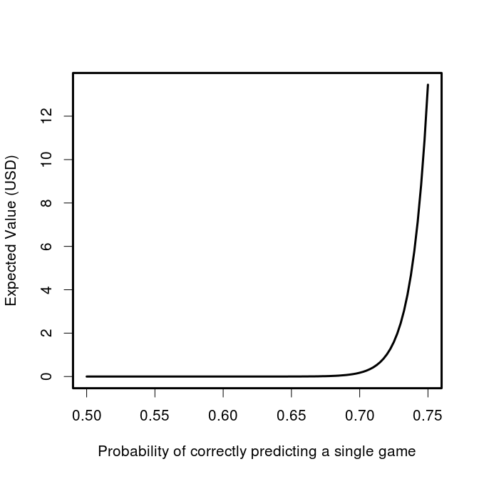
What level of predictiveness would you need to make this bet worth while? Let’s have a look at the expected value as a function of our individual game probability of being correct.

buffet1

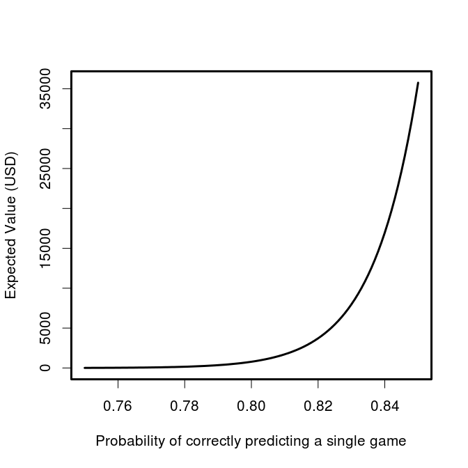
And if you think that you’re really good, we can look at the 0.75 to 0.85 range:

buffet2

So it’s starting to look enticing, you might even be willing to take off work for a while if you thought you could get your model up to a consistent 85% correct game predictions, giving you an expected return of ~$35,000. A recent paper found that even after observing the first 40 scoring events, the outcome of NBA games is only predictable at 80%. In order to be eligible to win, you’ve obviously got to submit your picks before the playoff games begin, but even at this herculean level of accuracy, the expected value of an entry in the contest plummets down to $785.

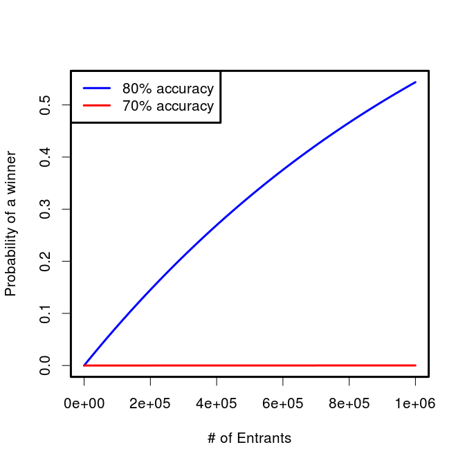
Those are the odds for an individual entrant, but what are the chances that Buffet and co will have to pay out? That, of course, depends on the number of entrants. Lets assume that the skill of all entrants is the same, though they all have unique models which make different predictions. In this case we can get the probability of at least one of them hitting it big. It will be the complement of no one winning. We already know the odds for a single entrant with a given level of accuracy, so we can just take the probability that each one doesn’t win, then take 1 minus that value.

buffet3

Just as we saw that the expected value is very sensitive to the predictive accuracy of the participant, so too is the probability that the prize will be awarded at all. If 1 million super talented sporting sages with 80%  game-level accuracy enter the contest, there will only be a slightly greater than 50% chance of anyone actually winning. If we substitute in a more reasonable (but let’s face it, still wildly high) figure for participants’ accuracy of 70%, the chance becomes only 1 in 5739  (0.017%) that the top prize will even be awarded even with a 1 million strong entrant pool.

tl;dr You’re not going to win, but you’re still going to play.

If you want to reproduce the numbers and plots in this post, check out this gist.

Simudidactic

auto·di·dact n.
A self-taught person.
From Greek autodidaktosself-taught : auto-auto- + didaktostaught;

+

sim·u·late v.
To create a representation or model of (a physical system or particular situation, for example).
From Latin simulre, simult-, from similislike;

=
(If you can get past the mixing of Latin and Greek roots)

sim·u·di·dactic adj.
To learn by creating a representation or model of a physical system or particular situation. Particularly, using in silico computation to understand complex systems and phenomena.

———————————————————————

This concept has been floating around in my head for a little while. I’ve written before on how I believe that simulation can be used to improve one’s understanding of just about anything, but have never had a nice shorthand for this process.

Simudidactic inquiry is the process of understanding aspects of the world by abstracting them into a computational model, then conducting experiments in this model world by changing the underlying properties and parameters. In this way, one can ask questions like:

  1. What type of observations might we make if x were true?
  2. If my model of the process is accurate, can I recapture the underlying parameters given the type of observations I can make in the real world? How often will I be wrong?
  3. Will I be able to distinguish between competing models given the observations I can make in the real world?

In addition to being able to ask these types of questions, the simudidact solidifies their understanding of the model by actually building it.

So go on, get simudidactic and learn via simulation!

simudidactic

Calculating AUC the hard way

The Area Under the Receiver Operator Curve is a commonly used metric of model performance in machine learning and many other binary classification/prediction problems. The idea is to generate a threshold independent measure of how well a model is able to distinguish between two possible outcomes. Threshold independent here just means that for any model which makes continuous predictions about binary outcomes, the conversion of the continuous predictions to binary requires making the choice of an arbitrary threshold above which will be a prediction of 1, below which will be 0.

AUC gets around this threshold problem by integrating across all possible thresholds. Typically, it is calculated by plotting the rate of false positives against false negatives across the range of possible thresholds (this is the Receiver Operator Curve)  and then integrating (calculating the area under the curve). The result is typically something like this:

auc

I’ve implemented this algorithm in an R script (https://gist.github.com/cjbayesian/6921118) which I use quite frequently. Whenever I am tasked with explaining the meaning of the AUC value however, I will usually just say that you want it to be 1 and that 0.5 is no better than random. This usually suffices, but if my interlocutor is of the particularly curious sort they will tend to want more. At which point I will offer the interpretation that the AUC gives you the probability that a randomly selected positive case (1) will be ranked higher in your predictions than a randomly selected negative case (0).

Which got me thinking – if this is true, why bother with all this false positive, false negative, ROC business in the first place? Why not just use Monte Carlo to estimate this probability directly?

So, of course, I did just that and by golly it works.

source("http://polaris.biol.mcgill.ca/AUC.R")
bs<-function(p)
{
 U<-runif(length(p),0,1)
 outcomes<-U<p
 return(outcomes)
}

# Simulate some binary outcomes #
n <- 100
x <- runif(n,-3,3)
p <- 1/(1+exp(-x))
y <- bs(p)

# Using my overly verbose code at https://gist.github.com/cjbayesian/6921118
AUC(d=y,pred=p,res=500,plot=TRUE)

## The hard way (but with fewer lines of code) ##
N <- 10000000
r_pos_p <- sample(p[y==1],N,replace=TRUE)
r_neg_p <- sample(p[y==0],N,replace=TRUE)

# Monte Carlo probability of a randomly drawn 1 having a higher score than
# a randomly drawn 0 (AUC by definition):

rAUC <- mean(r_pos_p > r_neg_p)
print(rAUC)

By randomly sampling positive and negative cases to see how often the positives have larger predicted probability than the negatives, the AUC can be calculated without the ROC or thresholds or anything. Now, before you object that this is necessarily an approximation, I’ll stop you right there – it is.  And it is more computationally expensive too. The real value for me in this method is for my understanding of the meaning of AUC. I hope that it has helped yours too!

Time-series forecasting: Bike Accidents

About a year ago I posted this video visualization of all the reported accidents involving bicycles in Montreal between 2006 and 2010. In the process I also calculated and plotted the accident rate using a monthly moving average. The results followed a pattern that was for the most part to be expected. The rate shoots up in the spring, and declines to only a handful during the winter months.

It’s now 2013 and unfortunately our data ends in 2010. However, the pattern does seem to be quite regular (that is, exhibits annual periodicity) so I decided to have a go at forecasting the time series for the missing years. I used a seasonal decomposition of time series by LOESS to accomplish this.

You can see the code on github but here are the results. First, I looked at the four components of the decomposition:

decomp_collisions

Indeed the seasonal component is quite regular and does contain the intriguing dip in the middle of the summer that I mentioned in the first post.

seasonal_collisions


This figure shows just the seasonal deviation from the average rates. The peaks seem to be early July and again in late September. Before doing any seasonal aggregation I thought that the mid-summer dip may correspond with the mid-August construction holiday, however it looks now like it is a broader summer-long reprieve. It could be a population wide vacation effect.

Finally, I used an exponential smoothing model to project the accident rates into the 2011-2013 seasons.

forecast_collisions

It would be great to get the data from these years to validate the forecast, but for now lets just hope that we’re not pushing up against those upper confidence bounds.

From Whale Calls to Dark Matter: Competitive Data Science with R and Python

Back in June I gave a fun talk at Montreal Python on some of my dabbling in the competitive data science scene. The good people at Savior-fair Linux recorded the talk and have edited it all together into a pretty slick video. If you can spare twenty-minutes or so, have a look.

If you want the slides, head on over to my speakerdeck page.

whaledarkmattercover

Uncertainty matters

In a post I wrote earlier this year, I noted a sentiment expressed in The Economist about understanding and embracing uncertainty.

…recent reforms to the IPCC’s procedures will do little to change its tendency to focus on the areas where there is greater consensus, avoiding the uncertainties which, though unpalatable for scientists, are important to policy. (link)

Which I felt was contrary to the way we, as scientists, speak among ourselves about policy makers. Specifically, that it is they who fear and misunderstand the implications of uncertainty.

This is the same perception which has led to the launch today by the group Sense About Science of a publication titled Making Sense of Uncertainty: Why uncertainty is part of science.

Launching a guide to Making Sense of Uncertainty at the World Conference of Science Journalists today, researchers working in some of the most significant, cutting edge fields say that if policy makers and the public are discouraged by the existence of uncertainty, we miss out on important discussions about the development of new drugs, taking action to mitigate the impact of natural hazards, how to respond to the changing climate and to pandemic threats.

Interrogated with the question ‘But are you certain?’, they say, they have ended up sounding defensive or as though their results are not meaningful. Instead we need to embrace uncertainty, especially when trying to understand more about complex systems, and ask about operational knowledge: ‘What do we need to know to make a decision? And do we know it?’

The report seems to be in line with arguments I have made about uncertainty and decision making as they pertain to ecological research, management, and policy.

Among the contributors to the report is someone who I consider to be among the best when it comes to understanding and communicating uncertainty, David Spiegelhalter. While I haven’t made my way all the way through it yet, it looks like this report will be an informative read for both scientists and policy makers (oh ya, and journalists — can’t forget about them).

Who knows, we might be able to stop the finger pointing and work together in mutual understanding of the importance of uncertainty.