Weapons of Math Destruction – A Data Scientist’s Guide to Disarmament

I’ve had this book on pre-order since spring and it finally arrived on Friday. I subsequently devoured it over the weekend.

Long awaited Weapons of Math Destruction by Cathy O'Neil

The book lays out a clear and compelling case for how data-driven algorithms can become — in contrast to their promise of amoral objectivism — efficient means for reproducing and even exacerbating social inequalities and injustices. From predictive policing and recidivism risk models to targeted marketing for predatory loans and for-profit universities, O’Neil explains how to recognize WMDs by 3 distinct features:

  1. The model is either hidden, or opaque to the individuals affected by its calculations, restricting any possibility of seeking recourse against – or understanding of – its results or conclusions.
  2. The model works against the subject’s interest (eg. it is unfair).
  3. The model scales, giving it the opportunity to negatively affect a very large segment of the population.

The taxonomy provides a simple framework for identifying WMDs in the wild. However, importantly for data scientists and other data practitioners, it forms a checklist (or rather an anti-checklist) to keep in mind when developing models that will be deployed into the real world. As data scientists, many of us are strongly incentivized to achieve feature 3, and doing so only makes it increasingly important to be constantly questioning the degree to which our models could fall victim to features 2 and 1.

Feature 2, as O’Neil lays out, can occur despite the best intentions of a model’s creators. This can (and does!) happen in two ways: First, when a modeler seeks to create an objective system for rating individuals (say, for acceptance to a prestigious university, or for a payday loan), the data used to build the model is already encoded with the socially constructed biases of the conditions under which it was generated. Even when attempting to exclude potentially bias-laden factors such as race or gender, this information seeps into the model nonetheless via correlations to seemingly benign variables such as zip codes or the makeup of a subject’s social connections.

Second, when the outcome of the model results in the reinforcement of the unjust conditions from which it was created, a negative feedback loop is created. Such a negative feedback loop is particularly present and pernicious in the use of recidivism risk models to guide sentencing decisions. An individual may be labeled as high risk due not to qualities of the individual himself, but his circumstances of living in a poor, high crime neighborhood. Being incarcerated based on the results of this model renders him more likely to end up back in that neighborhood, subject to continued poverty and disproportionate policing. Thus the model has set up the conditions to fulfill its own prediction.

As machine learning algorithms become more and more accurate at a variety of tasks, their inner workings become harder and harder to understand. The trend will make it increasingly difficult to avoid feature 1 of the WMD taxonomy. Current advanced techniques like deep learning are creating models that are remarkably performant, yet not fully understood by the researchers creating them, much less the individuals affected by their results. In light of this, we need to think carefully as data scientists about how to communicate these models with as much transparency as possible. How to do so remains an open question. But the internal ‘black box’ nature of these algorithms does not obviate our responsibility to disclose exactly what input data went into a given model, what assumptions were made of that data, and on what criteria the model was trained.

Overall, WMD provides an incredibly important framework for thinking about the consequences of uncritically applying data and algorithms to people’s lives. For those of us, like O’Neil herself, who make our living using mathematics to create data-driven algorithms, taking to heart the lessons contained in Weapons Of Math Destruction will be our best defense against unwittingly creating the bomb ourselves.

Advertisement

Time-series forecasting: Bike Accidents

About a year ago I posted this video visualization of all the reported accidents involving bicycles in Montreal between 2006 and 2010. In the process I also calculated and plotted the accident rate using a monthly moving average. The results followed a pattern that was for the most part to be expected. The rate shoots up in the spring, and declines to only a handful during the winter months.

It’s now 2013 and unfortunately our data ends in 2010. However, the pattern does seem to be quite regular (that is, exhibits annual periodicity) so I decided to have a go at forecasting the time series for the missing years. I used a seasonal decomposition of time series by LOESS to accomplish this.

You can see the code on github but here are the results. First, I looked at the four components of the decomposition:

decomp_collisions

Indeed the seasonal component is quite regular and does contain the intriguing dip in the middle of the summer that I mentioned in the first post.

seasonal_collisions


This figure shows just the seasonal deviation from the average rates. The peaks seem to be early July and again in late September. Before doing any seasonal aggregation I thought that the mid-summer dip may correspond with the mid-August construction holiday, however it looks now like it is a broader summer-long reprieve. It could be a population wide vacation effect.

Finally, I used an exponential smoothing model to project the accident rates into the 2011-2013 seasons.

forecast_collisions

It would be great to get the data from these years to validate the forecast, but for now lets just hope that we’re not pushing up against those upper confidence bounds.

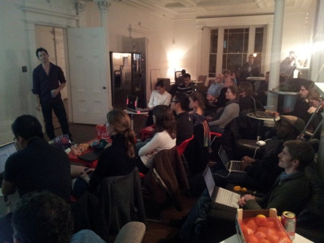
What does R do? Bring people together, of course!

Last night we had a great meet up of the Montreal R User Group. I got things started with a little presentation asking the question “What does R do?” (slides). I made the presentation using Montreal R User Group member Ramnath Vaidyanathan‘s Slidify package. Slidify allows you to generate rather handsome HTML5 slides directly using R markdown.

We were then treated to a great workshop by Etienne Low-Decarie. He gave us a fly over of some of the most powerful R packages for wrangling data, namely plyr, reshape and ggplot.

Here are Etienne’s slides.

You can also follow along with the code posted here.

We met a lot of people who are doing very cool things using R. I’m looking forward to our next meetup!

I’m no shutterbug – drop me a note if you came and have any better pictures.

We had clementines!

Also, thanks to Notman House for hosting us. The haunted house feeling wasn’t enough to scare off this hardy group of data geeks.

Mapping Bike Accidents in R

At last weekend’s Hack Ta Ville event here in Montreal, I joined up with some talented urban planners and web devs to realize Vélobstacles. The idea of the project is to crowd source information on cycling conditions around the city. As with any crowd sourcing project, we were faced with the problem of seeding the site with some data to draw the attention of users to get the ball rolling.

Fortunately, we had access to a data set of all reported cycling accidents between 2006-2010. Once we seeded Vélobstacles with this data, the web devs went to town adding features to the site, and I had outlived my usefulness as a data geek. So I decided to play with the accident data a little and produce some visualization. I plotted all the accidents on a map and animated it through time. I also calculated and plotted the monthly accident rate using a moving average.

Be sure to select HD quality:

Not surprisingly, the accident rate goes way up in the summer months as Montreal winters are braved on two wheels by only a rarefied few. What is interesting is the mid-summer dip in the accident rate. This dip is notably correlated with Montreal’s much beloved construction holiday – though the causal relationship is unclear. If you have any alternative explanations, or an idea about how to test the construction holiday hypothesis, drop a note in the comments.

As always, you can get the code on my github page.

Real-time data collection and analysis in class

As September draws nearer, my mind inevitably turns away from my lofty (and largely unmet) summer research goals, and toward teaching.  This semester I will be trying out a teaching technique using live data collection and analysis as a tool to encourage student engagement.  The idea is based on the electronic polling technology known as ‘clickers‘. The technology allows you to get instant feedback from students, check for understanding, and when used appropriately it can facilitate active engagement and peer learning.

Because I will be teaching in a computer lab, where all of the students will be sitting at a computer, I have the advantage of being able to bypass the little devices, and instead gather student responses using a web based interface.  The advantages, as I see them, are:

  1. Students can enter more complex input than the 1-9 provided by clickers. Instead, students can enter any number or character vector response.
  2.  Students can instantly download, plot, and analyze the class data.  This step is facilitated by the read.csv("http://data_url.csv") function in R, which allows data import directly from the web.

The first exercise I have planned using this technology is to have students enter their height, then have them plot a histogram of the data to introduce the normal distribution.  Using the simple online interface I have created, this exercise can be done very quickly. I am calling the tool I am one of n.

If you have any suggestions for learning activities that could make effective use of this technology in an undergraduate Biostatistics (or other) course, drop me a note!