The Treachery of Models

In Magritte’s famous 1929 painting The Treachery of Images, a pipe is depicted with the caption “Ceci n’est pas une pipe“, French for “This is not a pipe”. The seemingly dissonant statement under what is a very clearly depicted pipe forces the viewer to confront the distinction between the representation and the thing itself. The treachery refers to the danger involved in confusing the representation with the object.

Models – like images – are merely representations of the objects they depict. The modeler seeks to represent the relevant properties of the system being modeled in order to communicate some features of that system, or to manipulate it under ‘what-if’ scenarios.

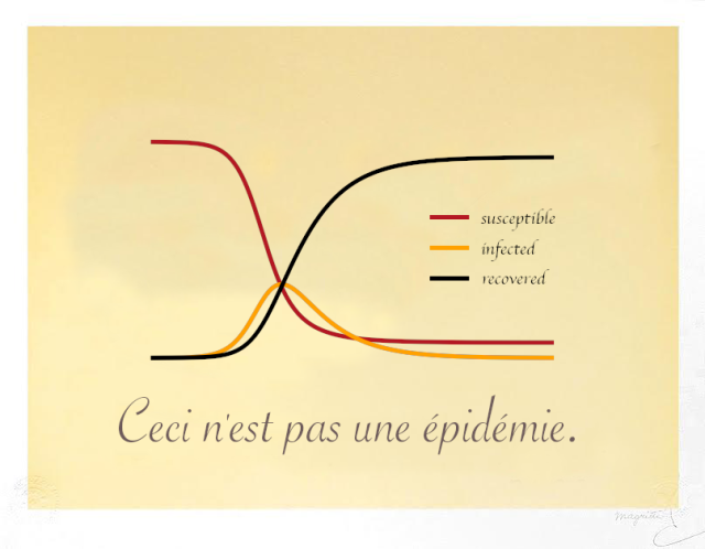
With the current plethora of models of COVID-19 spread, it seems important to remind ourselves of Magritte’s warning. Models can be incredible tools — abstractions of complex realities that allow us to reason about the data we’ve seen so far, and consider possible futures. But they are not the epidemic process itself.

Ceci n'est pas une épidémie.

This is not an argument that the models themselves are treacherous. I absolutely adore modeling and models, as Magritte adored painting and images. I consider modeling an essential tool to further our understanding of (and make predictions about) the world around us. Indeed I developed one of the aforementioned COVID-19 models with my colleagues at Penn Medicine. The treachery comes when we mistake the abstraction for reality.

Germination Project Fellows come to Penn

I was recently fortunate to be invited to speak with an impressive group of high-school students as a part of the Germination Project. They came to Penn to learn about innovation in health care and I spoke with them about how we’re using Data Science to improve patient outcomes.germination_talk_screenshot

Visualizing classifier thresholds

Lately I’ve been thinking a lot about the connection between prediction models and the decisions that they influence. There is a lot of theory around this, but communicating how the various pieces all fit together with the folks who will use and be impacted by these decisions can be challenging.

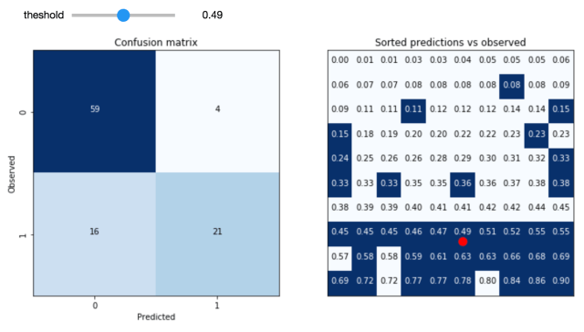
One of the important conceptual pieces is the link between the decision threshold (how high does the score need to be to predict positive) and the resulting distribution of outcomes (true positives, false positives, true negatives and false negatives). As a starting point, I’ve built this interactive tool for exploring this.

Screen Shot 2017-11-13 at 11.16.26 AM

The idea is to take a validation sample of predictions from a model and experiment with the consequences of varying the decision threshold. The hope is that the user will be able to develop an intuition around the tradeoffs involved by seeing the link to the individual data points involved.

Code for this experiment is available here. I hope to continue to build on this with other interactive, visual tools aimed at demystifying the concepts at the interface between predictions and decisions.

Weapons of Math Destruction – A Data Scientist’s Guide to Disarmament

I’ve had this book on pre-order since spring and it finally arrived on Friday. I subsequently devoured it over the weekend.

Long awaited Weapons of Math Destruction by Cathy O'Neil

The book lays out a clear and compelling case for how data-driven algorithms can become — in contrast to their promise of amoral objectivism — efficient means for reproducing and even exacerbating social inequalities and injustices. From predictive policing and recidivism risk models to targeted marketing for predatory loans and for-profit universities, O’Neil explains how to recognize WMDs by 3 distinct features:

  1. The model is either hidden, or opaque to the individuals affected by its calculations, restricting any possibility of seeking recourse against – or understanding of – its results or conclusions.
  2. The model works against the subject’s interest (eg. it is unfair).
  3. The model scales, giving it the opportunity to negatively affect a very large segment of the population.

The taxonomy provides a simple framework for identifying WMDs in the wild. However, importantly for data scientists and other data practitioners, it forms a checklist (or rather an anti-checklist) to keep in mind when developing models that will be deployed into the real world. As data scientists, many of us are strongly incentivized to achieve feature 3, and doing so only makes it increasingly important to be constantly questioning the degree to which our models could fall victim to features 2 and 1.

Feature 2, as O’Neil lays out, can occur despite the best intentions of a model’s creators. This can (and does!) happen in two ways: First, when a modeler seeks to create an objective system for rating individuals (say, for acceptance to a prestigious university, or for a payday loan), the data used to build the model is already encoded with the socially constructed biases of the conditions under which it was generated. Even when attempting to exclude potentially bias-laden factors such as race or gender, this information seeps into the model nonetheless via correlations to seemingly benign variables such as zip codes or the makeup of a subject’s social connections.

Second, when the outcome of the model results in the reinforcement of the unjust conditions from which it was created, a negative feedback loop is created. Such a negative feedback loop is particularly present and pernicious in the use of recidivism risk models to guide sentencing decisions. An individual may be labeled as high risk due not to qualities of the individual himself, but his circumstances of living in a poor, high crime neighborhood. Being incarcerated based on the results of this model renders him more likely to end up back in that neighborhood, subject to continued poverty and disproportionate policing. Thus the model has set up the conditions to fulfill its own prediction.

As machine learning algorithms become more and more accurate at a variety of tasks, their inner workings become harder and harder to understand. The trend will make it increasingly difficult to avoid feature 1 of the WMD taxonomy. Current advanced techniques like deep learning are creating models that are remarkably performant, yet not fully understood by the researchers creating them, much less the individuals affected by their results. In light of this, we need to think carefully as data scientists about how to communicate these models with as much transparency as possible. How to do so remains an open question. But the internal ‘black box’ nature of these algorithms does not obviate our responsibility to disclose exactly what input data went into a given model, what assumptions were made of that data, and on what criteria the model was trained.

Overall, WMD provides an incredibly important framework for thinking about the consequences of uncritically applying data and algorithms to people’s lives. For those of us, like O’Neil herself, who make our living using mathematics to create data-driven algorithms, taking to heart the lessons contained in Weapons Of Math Destruction will be our best defense against unwittingly creating the bomb ourselves.

Introduction to Machine Learning Talk

There was an amazing turnout at last night’s DataPhilly meetup (~200 people!). I was completely delighted by the turnout and people’s engagement level. Here are the slides of the talk I gave to set up the evening with a high-level introduction to machine learning.


A probabilistic justification to carpe diem

There’s a curious thing about unlikely independent events: no matter how rare, they’re most likely to happen right away.

Let’s get hypothetical

You’ve taken a bet that pays off if you guess the exact date of the next occurrence of a rare event (p = 0.0001 on any given day i.i.d). What day do you choose? In other words, what is the most likely day for this rare event to occur?

Setting aside for now why in the world you’ve taken such a silly sounding bet, it would seem as though a reasonable way to think about it would be to ask: what is the expected number of days until the event? That must be the best bet, right?

We can work out the expected number of days quite easily as 1/p = 10000. So using the logic of expectation, we would choose day 10000 as our bet.

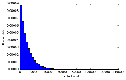
Let’s simulate to see how often we would win with this strategy. We’ll simulate the outcomes by flipping a weighted coin until it comes out heads. We’ll do this 100,000 times and record how many flips it took each time.

p0001

The event occurred on day 10,000 exactly 35 times. However, if we look at a histogram of our simulation experiment, we can see that the time it took for the rare event to happen was more often short, than long. In fact, the event occurred 103 times on the very first flip (the most common Time to Event in our set)!

So from the experiment it would seem that the most likely amount of time to pass until the rare event occurs is 0. Maybe our hypothetical event was just not rare enough. Let’s try it again with p=0.0000001, or an event with a 1 in 1million chance of occurring each day.

p0000001

While now our event is extremely unlikely to occur, it’s still most likely to occur right away.

Existential Risk

What does this all have to do with seizing the day? Everything we do in a given day comes with some degree of risk. The Stanford professor Ronald A. Howard conceived of a way of measuring the riskiness of various day-to-day activities, which he termed the micromort. One micromort is a unit of risk equal to p = 0.000001 (1 in a million chance) of death. We are all subject to a baseline level of risk in micromorts, and additional activities may add or subtract from that level (skiing, for instance adds 0.7 micromorts per day).

While minimizing the risks we assume in our day-to-day lives can increase our expected life span, the most likely exact day of our demise is always our next one. So carpe diem!!

Post Script:

Don’t get too freaked out by all of this. It’s just a bit of fun that comes from viewing the problem in a very specific way. That is, as a question of which exact day is most likely. The much more natural way to view it is to ask, what is the relative probability of the unlikely event occurring tomorrow vs any other day but tomorrow. I leave it to the reader to confirm that for events with p < 0.5, the latter is always more likely.

Simudidactic

auto·di·dact n.
A self-taught person.
From Greek autodidaktosself-taught : auto-auto- + didaktostaught;

+

sim·u·late v.
To create a representation or model of (a physical system or particular situation, for example).
From Latin simulre, simult-, from similislike;

=
(If you can get past the mixing of Latin and Greek roots)

sim·u·di·dactic adj.
To learn by creating a representation or model of a physical system or particular situation. Particularly, using in silico computation to understand complex systems and phenomena.

———————————————————————

This concept has been floating around in my head for a little while. I’ve written before on how I believe that simulation can be used to improve one’s understanding of just about anything, but have never had a nice shorthand for this process.

Simudidactic inquiry is the process of understanding aspects of the world by abstracting them into a computational model, then conducting experiments in this model world by changing the underlying properties and parameters. In this way, one can ask questions like:

  1. What type of observations might we make if x were true?
  2. If my model of the process is accurate, can I recapture the underlying parameters given the type of observations I can make in the real world? How often will I be wrong?
  3. Will I be able to distinguish between competing models given the observations I can make in the real world?

In addition to being able to ask these types of questions, the simudidact solidifies their understanding of the model by actually building it.

So go on, get simudidactic and learn via simulation!

simudidactic

What is probabilistic truth? Part 2 – Everything is conditional

Read Part 1

When making a statement of the form “1/2 is the correct probability that this coin will land tails”, there are a few things which are left unsaid, but which are typically implied.

The statement is one about the probability of an unknown event occurring, and it would seem reasonable to write this statement using probability notation as P(toss=tails) = 0.5. And indeed many people would express it this way. However, what is missing is the state of knowledge under which this statement has been made. For instance, is the coin yet to be flipped, or is it currently rolling in a circle on the table, leaning in toward its final resting position? Perhaps the flipping device can consistently throw a coin such that it rotates exactly 5 times in the air before landing flat on the table, or we know which side is up at the start of the flip. In these latter cases, the statement of probability would be made under considerably more knowledge than the first, and would not tend to be 0.5 in these cases. An observer placing a probability of P(toss=tails) = 0.99 at the moment when the coin is circling in on its resting position, leaning heavily toward a tails up configuration, could be said to have the correct probability also. For fairness, lets say that the first observer also makes her probability statement at the same moment, but from another room where she cannot see what has happened.

How can P(toss=tails) = 0.5, and P(toss=tails) = 0.99 be simultaneously correct?

The answer is conditioning. Each of the statements were made conditional on the observer’s state of knowledge. More completely, the two statements can be rewritten as:

P(toss=tails | knowledge of observer 1) = 0.5 , and

P(toss=tails | knowledge of observer 2) = 0.99

In practice, however, we often leave out the conditional part of the notation unless it is germane to the problem at hand. However, there is no such thing as unconditional probability. In fact, Harvard professor Joe Blitzstein calls conditioning the Soul of Statistics.

In the next post in this series, we’ll start looking at how to assess the correctness of a (conditional) probability statement after having observed an outcome.

Here's a bunch of random walks -- just 'cause its neat.

Here’s a bunch of random walks — just ’cause its neat.

Simulation and Likelihood Methods Workshop in Kananaskis

I can think of worse places to get down and dirty with R than Kananaskis, Alberta.

Zero to R Hero

CAISN_Primary_trans

Canadian Aquatic Invasive Species Networks Annual General Meeting in Kananaskis, Alberta. May 03, 3:25-5:30.

This 2-hour workshop will focus on how and why we do numerical simulation in R. Time permitting, we will also look at how to build and fit likelihood based statistical models.

We ask that you bring your laptop with both R and R-Studio installed. If you’ve never worked with R before, please have a look at the getting started with R document. You can
also check out the slides from our more introductory workshops.

Outline

Section 1: Introduction to Simulation (script)

  •     What is (numerical) simulation?
  •     Drawing random samples from a set
  •     Drawing random samples from a probability distribution
  •     Describing models in terms of their deterministic and stochastic parts
  •     Simulating data from a model

Section 2: Likelihood Methods(script)

  •     The Likelihood Principle
  •     The Ecologist’s Quarter
  •     Maximum…

View original post 30 more words

Mathematical abstraction and the robustness to assumptions

I’ve been showing my new favourite toys to just about anyone foolish enough to actually engage me in conversation. I described how my shiny new set of non-transitive dice work here, complete with a map showing all the relevant probabilities.

All was neat and tidy and wonderful until fellow ecologist, Aaron Ball, tried to burst my bubble.

Nope. I couldn’t find the error. Fortunately, he works across the hall so I just went and asked him.

The problem he found, it turns out, was not with my calculations but with my assumptions. Aaron told me that dice constructed with rounded corners and hollowed out pips for the numbers on the faces tend to be biased in the frequency at which each face rolls up. I had assumed, of course, that each side of each of the five dice would roll with the same probability (ie. 1 in 6).

As with any model of a real world system, the mathematics were carried out on a simplified abstraction of the system being modelled. There are always, by necessity, assumptions being made. The important thing is to make these assumptions as explicit as possible and, where possible, to test the robustness of the model predictions to violations of the assumptions. Implicit to my calculations of the odds of the non-transitive Grime dice was the assumption that the dice are fair.

To check the model for robustness to this assumption, we can relax it and find out if we still get the same behaviour. Specifically, we can ask here whether some sort of pip-and-rounded-corner-induced bias can lead to a change in the Grime dice non-transitive cycles.

It seems a natural place to look would be between the dice pairings which have the closest to even odds. We can find out what level of bias would be required to switch the directionality of the odds (or at least erase the tendency for one die to roll higher than the other). Lets try looking at Magenta and Red, which under the fair dice assumption have odds p(Magenta > Red)=5/9. What kind of bias will change this relationship? The odds can be evened out by either Magenta rolling ones more often, or red rolling nine more often. The question is then, how much bias would there need to in the dice in order to even out the odds between Magenta and Red?

Lets start with Red biasing toward rolling nine more often (recall that nine appears on only one face). Under the fair dice hypothesis, Red can roll nine (1/6 of the time) and win no matter what Magenta rolls, or by rolling four (5/6 of the time) and win when Magenta rolls one (1/3 of the time).

P(Red > Magenta) = 1/6 + 5/6 * 1/3, which is 4/9.

If we set this probability equal to 1/2, and replace the fraction of times that Red rolls nine with x, we can solve for the frequency needed to even the odds.

x + 5/6 * 1/3 = 1/2

x = 2/9

Meaning that the Red die would have to be biased toward rolling nine with 2/9 odds. That’s equivalent to rolling a nine 1 and 1/3 times (33%) more often than you would expect if the die were fair!

Alternatively, the other way the odds between Red and Magenta could be evened is if Magenta biased towards rolling ones more often. We can do the same kind of calculation as above to figure out how much bias would be needed.

1/6 + 5/6 * x = 1/2

x = 2/5

Which corresponds to Magenta having  a 20% bias toward rolling ones. Of course, some combination of these biases could also be possible.

I leave it to the reader to work out the other pairings, but from the Red-Magenta analysis we can see that even if the dice deviated quite a bit from the expected 1/6 probability for each side, the edge afforded to Magenta is retained. I couldn’t find any convincing  evidence for the extent of bias caused by pipping and rounded corners but it seems unlikely that it would be strong enough to change the structure of the game.