In February, I was honoured with the inaugural McGill Biology Graduate Students Association Organismal Seminar Award. This is the talk I gave on uncertainty and predictions in ecological management. I have inserted selected visuals, but you can get the complete slides which accompanied the talk here.

———————————————————————————————————–

Predictive invasion ecology and management decisions under uncertainty

When I was told that I had been selected to give this talk I spent a rather long time thinking about how one goes about preparing a presentation of this type. The typical graduate student experience presenting at a conference is that we are expected to detail a single piece of research to a relatively small audience of fellow researchers who, it is hoped, have at least a tertiary familiarity with whatever esoteric domain we’ve been recently slaving away in. The format usually goes: Introduction – methods – results – conclusion – next speaker. However, it seemed to me that if I was going to ask you all to come out and listen during what would otherwise be a prime manuscript writing Thursday afternoon, I was going to have to do something a little different, and I hope, more interesting.

I’ve titled the talk ‘Predictive invasion ecology and management decisions under uncertainty’, and indeed that is what I’ll be talking about. However, I’ve decided to structure this talk as something more akin to an argumentative essay. And the argument that I am going to be making has to do with how, as I see it, we should be doing ecology as it pertains to informing management and policy decisions.

By this I mean, how do we go from data, which is often sparse or limited, and theory, which is our (also limited) abstracted understanding of ecological processes, to making inference, predictions, and ultimately, to help inform decisions. I am going to lay out, and advocate, a framework for how I think that we ought to go about this. I’ll outline a sort of methodological recipe for doing this, and then I’ll go through how I have applied this general methodological approach in my own research. First on measuring the impacts of invasive species (specifically forest pests), then on various aspects of the spread, and management, of aquatic invasives.

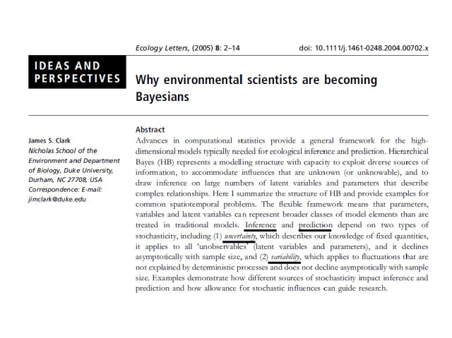
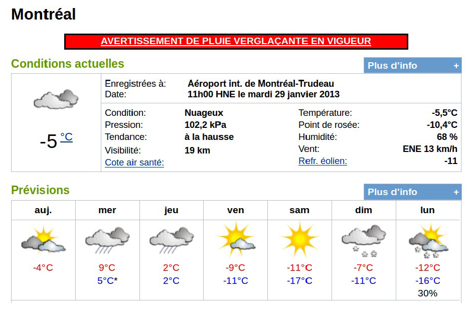
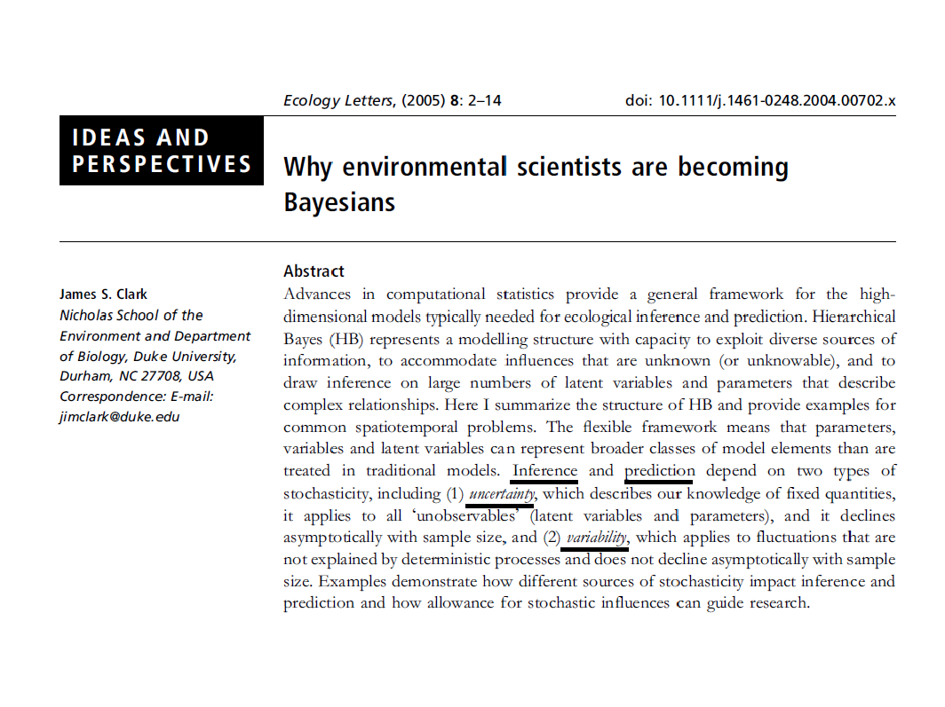
The paper that I gave to Carly to send around as recommended reading (which I’m sure you all diligently read), is this one. This is one of the first papers that I came across when I started graduate work here at McGill. Clark and colleagues published this paper in Science back in 2001, but its message is just as, if not more important today. In it, the authors argue that if we are going to make decisions about what to do to conserve biological diversity, ecosystem function, and the valuable ecosystem services provided to use by nature, then we will need to make forecasts about what we expect to happen in the future. I was struck by something that Justin Travis said last week during his talk about the idea of engaging in ‘ecological meteorology’. Which might bring to mind something like this.

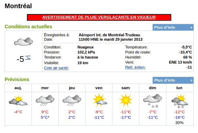
When we think of forecasting, we usually think about the best guess at what some future state of nature is going to be. When I speak of forecasts, however, I mean something a little bit different than what is communicated by weather forecasters. When I talk about forecasting, I mean specifically placing probability distributions over the range of possible future outcomes, and in that sense, a forecast is not a single prediction about a future state of nature, but rather is a way to communicate uncertainty about the future. And indeed, our level of uncertainty may well be quite high. It was the Danish physicist Niels Bohr, who once said:

Prediction is very difficult, especially about the future.

–Niels Bohr, Danish physicist (1885-1962)

Now, the temptation can be to suggest that because this is true, we should not act. Many will call for ‘further study’, or cite ‘insufficient data available’ as a reason to delay decisions. Of course, we can always collect more data, and we there is always room to further refine and develop our theory and models. And yes, indeed, we ought to continue to do both of these things. However, the approach of not making a decision has been thought of as being a precautionary one, on the basis that action can have unintended consequences. I want to outline why I believe that this is not the correct way to think about things.

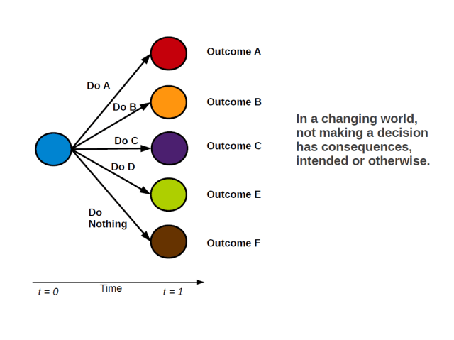
1. Not making a decision is, itself a decision!
2. As such, in a changing world, doing nothing can also have unintended consequences!

Delaying decision making on the hopes that things with stay the same, may very well have the unintended consequence that they will not. By doing away with this we can focus on the problem at hand. And that is: How do make the best use of the data that we have to make predictions which take into account (potentially large) inherent uncertainties?

That is, how do we use all of the information that we have available to us to make probabilistic predictions, with their many sources of uncertainty, about the things that we are interested in? For instance, in my own work, these are things like: How much damage are non-native forest insects causing, and how much damage should we expect to be caused by the next one? At current import rates, what is the probability of a new fish species invading via the aquarium trade? Or, after initial introduction, how is a novel invasive likely to spread across the landscape? And how is that spread likely to be altered in the presence of targeted mitigation strategies?

The framework that I am advocating approaches all of these problems in a similar way. At this point, for those of you who know me, you’re probably making a guess about where I’m going here.

Here again is Jim Clark, this time outlining all the wonderful things that the Bayesian can do. Bayes is indeed a useful tool for doing inference and prediction while accounting for uncertainty and variability. However, I am not going to argue here specifically for the use of Bayesian methods (though they can help.) In fact, in my own work I have used both classical maximum likelihood, as well as Bayesian methods to get the job done. Instead, I am arguing for the use of a broader framework. The important elements of this framework are that we use the information (data) that we have available to us to the maximum extent possible while taking account of our uncertainties in the form of probability distributions. It turns out that Bayesian methods are great at this. They do, however suffer from other problems, not the least of which can be the computational costs of estimating models.

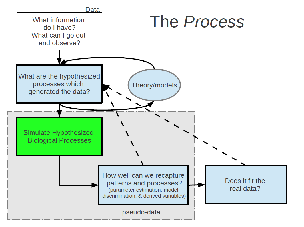
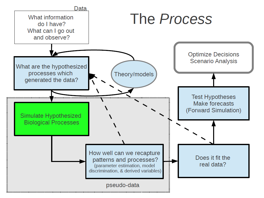
Let’s start outlining a procedure for this general methodological framework which I am proposing. The first step is data.

—> What information do I have? What can I go out and observe? <—

Some may suggest starting with theory, but I would argue that if the theory or models don’t make predictions about observable, quantifiable phenomena, then we’re done before we even get started. So, start with data. In ecology, we often have observational data (as a opposed to experimental data). From the information (or data) that we have, we can then start asking the question:

—> What are the hypothesized processes which generated these data? <—

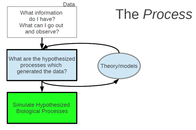
This is where our ecological understanding comes in in the form of models. Models are our abstractions of what we believe to be the key processes involved in some real world phenomenon. These abstractions of real world processes, by definition contain only a subset of the real components which are involved. Therefore, something we need to always keep in mind was best said by George Box:

All models are wrong, but some are useful.

–George E.P. Box.

This is a quote that I am sure many of you are familiar with, but I find it to be a very useful one to remind myself of from time to time. Any model or theory that we have of the world will be incomplete. The challenge we face is to build our abstractions of real world processes such that they contain the main relevant features of the phenomena that we are interested in, and produce predictions about observable quantities in the real world.

Once we have formalized our theories about how we think that our observable data is being generated into one or more models, the next step is to build an artificial world and in that world, to simulate the data generating process from your models.

By this I mean stochastic simulation – the in silico use of random number generation to probabilistically mimic the behaviour of individuals or populations. Random number generation is really the best thing since sliced bread. It can be used as a tool to generate and test theories and as a platform to conduct thought experiments about complex systems.

This is a step that I believe is most often skipped in studies with data. Many studies go straight from formulating a model to confronting that model with data. Instead, the next step should be to confront your model, or models, with the psuedo data, which is in the exact same form as your real world data.

I have found this step to be critically important as a safeguard against faulty logic. If you’re anything like me, you will have many of these moments when building and testing models.

A rather nefarious thing about models is that even broken ones can produce seemingly reasonable predictions when confronted with data. The point is that simulation provides a test suite (a massive laboratory right in your computer) for experimenting and testing your logic before confronting models with data.

Once we have gone around this loop a few (or many) times, only then do we go ahead and test it out on our real data. At this point you may still need to go back to the theoretical drawing board, but hopefully you’ve ironed out all the kinks in your logic. It is hear that you estimate model parameters and distinguish between competing models.

You are now ready to start testing hypotheses about how a system may behave if altered, and to make probabilistic forecasts about things you care about. Here, as a bonus, you’ve already set up a simulation model of your system which you can now use to push forward in time under any given scenario or intervention you may be considering.

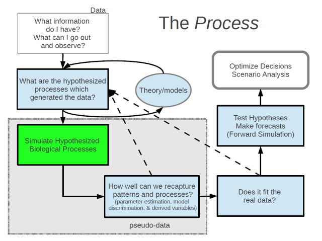
It is then possible to run all kinds of analyses of risk based on our probabilistic forecasts in order to help make decisions about management that will maximize our probability of getting a desired outcome.

I have presented this as a general framework that I think is applicable to broad range of ecological problems as a way to link data and theory to make inference, predictions and inform decisions under uncertainty. What I want to do now is to give you a look at how I’ve used this general methodological framework in my own research, which is specific to invasive species.

The first project that I worked on when I arrived for graduate study at McGill was on estimating the impacts of non-native forest insects in the US. I don’t know how I swung this one, but no sooner that I had arrived, Brian was bringing me down to California to work with an amazing interdisciplinary team of forest ecologists, entomologists, and resource economists on this project at NCEAS.

First a bit about invasive forest insects. We know that while international trade provides many economic benefits, there are also many externalities that are not taken into consideration. When we move massive amounts of stuff around the globe, we inevitably also move species, and some of these species can become problematic in their adoptive landscape. We know that some of these species are causing large ecological and economic damages, but we don’t really have any estimates of what the total damages are amounting to. Without any estimate, these damages can not be incorporated into the cost of trade, nor can we make informed decisions about what costs we would be willing to pay to avoid them.

Given that there are many non-native species being introduced and only a fraction of those are highly damaging, we also wanted to get an estimate of the probability of seeing another high impact pest under current import levels and phytosanitary legislation. Further, since the mode by which forest pests are being transported is highly associated with the feeding guild of the insects, we wanted to get separate estimates grouped by guild. And since economic impact is not likely to be evenly distributed, we set out to determine who is paying for these impacts.

So, what information did we have? Not much, really. The entomologists set out to compile a list of all known non-native forest pests, and to identify a short list of those species that had been documented to have caused some noticeable damage. While we would have liked them to have done all of the species, the lazy economists agreed to do a national scale, full cost analysis of the most damaging pest in each of the three feeding guilds (borers, sap suckers, and foliage feeders). And they did this analysis across three broad economic sectors (costs borne to government, households, and to the lumber market).

The information which we had then, for each guild and economic sector, was a count of the number of species causing very little damage (most of them), the number a species causing some intermediate level of damage (a few), and one estimate of the damage caused by the most damaging species.

How do we go from this information to an estimate of the frequency distribution of costs across all species? We assumed from what we know about there being many innocuous species, fewer intermediate species and only one real ‘poster’ species in each guild, that the distribution was likely to be concave across most of it’s range and that the frequency of species causing infinite damage should asymptote to zero.

There are only a handful of functional forms that meet our asymptotic and concavity assumptions, fitting distributions using maximum likelihood would be fairly straightforward. But unfortunately, what we have are frequencies of species in different ranges.

The solution to this is to integrate the curve in these ranges and use that integral in our likelihood function.

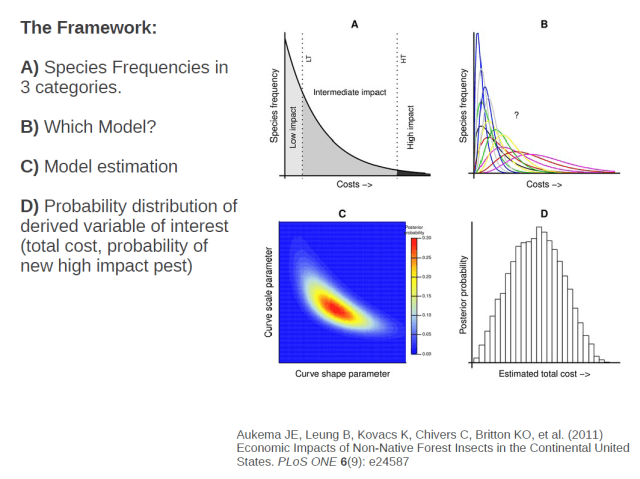
So to recap, we have counts of species in each of three cost categories. From that information we want to determine which functional form is likely to have generated that observed data. The parameters of each functional form themselves are uncertain, but we want to estimate a probability distribution of which values are more likely. And from there, with the distribution of possible distributions in hand, we can extract any number of useful quantities, for instance, the total cost of all species, the expected cost of a new species, or the probability that a new species will be a highly damaging one.

Okay, nice system, but will it work? To find out if our scheme would work, we simulated from each of the models, actually generating each data point, then collected ‘pseudo-data’ in the form which we actually had in real life, and went ahead to see if we could, in fact get back both the generating model, and the generating parameters.

The great thing about simulations is that you know what the model and parameters are that generated your simulated data. So when you apply your estimation procedures, you can assess how well you’ve done. So here we had four possible generating functional forms (power, log-normal, gamma, weibull), and what I check for is how often the estimating procedure is able to correctly identify the generating model. While some models were less distinct from others, we were able to in fact recapture the generating model.

We also check to see that we can recapture the parameter values and any derived quantities of interest. Again the panels are the four models, and in green are samples from the posterior distribution of parameter values with the generating value shown in red. Shown here is only one instance, but what we actually did was to re-simulate thousands of times to determine whether the generating parameter values were distributed as random draws from the posterior distribution. Since, for any one instance we wouldn’t expect the posterior distribution to be centred exactly on the true value, but rather that the true value would be a random draw from the posterior distribution.

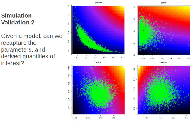
Also shown in these plots as a color ramp is the total cost associated with a curve having those parameter values. We also checked to ensure that there was no bias in our estimations of our derived quantities of interest.

I’m showing here the procedure that worked, however this took some doing to get right – highlighting the importance of testing models via simulation before sending out in prime-time.

So we found that the bulk of the cost of invasive forest insects was being placed on local governments, and that it was borers doing all the damage at around 1.7billion USD per annum. We also found that the single most damaging pest in each guild was responsible for between 25 and 50 % of the total impacts, and that at the current rates of introduction, there is about a 32% chance that another highly damaging pest will occur in the next 10 years.

Staying on the theme of imports, I want to move now to the live fish trade, and specifically invasion risk posed by aquarium fish. This is some work that is forthcoming in Diversity and Distributions which I did with lab mate, Johanna Bradie wherein we had some fairly high resolution data on fish species that were being imported to Canada. We had records of the number of individuals at the species level that were reported at customs, and we wanted to know ‘given only this information, can we estimate the risk of establishment?’.

So we know that due to species specific traits such as life history and environmental tolerances, that not all species are equally likely to establish. However, what we wondered was, in the absence of this information, can we estimate an overall pathway level risk. So if you look at the plot, what I am showing is that the relationship between propagule pressure and probability of establishment is not likely to be the same across different species. But the question is ‘how much does this matter in determining a risk estimate in the absence of species specific information?’

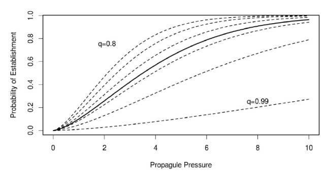
What we showed using simulation was that in most cases, it was possible to estimate a pathway level establishment curve, without significant bias. The only place where it particularly failed was when the distribution of q values, which is essentially a measure of environmental suitability, was strongly bimodal. Or, in other words, where there are two very different types of species represented in the import pool.

In short we found that at an import level of 100,000 individuals, there was pathway level establishment risk of 19%, and that importing 1 million individuals leads to just under a 1 in 2 chance of establishment for a species chosen at random from the import pool.

These studies so far have looked at invasions at very broad spatial scales, but now I want to drill down a little and talk about the process of species spread across a landscape once a local population has been established. Specifically, I investigate the way in which human behaviour mediates the dispersal of aquatic invasive species at the landscape level, and how these patterns of dispersal interact with the population dynamics of the invading species to affect the spatial patterns of spread.

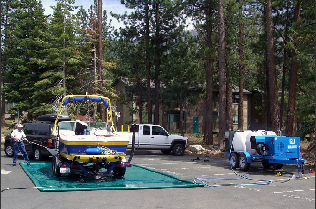
We’ve known for a while now that freshwater species are transported from lake to lake primarily by hitchhiking to recreational vessels like this one here. If we are going to try to make predictions about how species will spread, it stands to reason that we should probably try to understand the behaviour of the humans who are pulling these boats around. There have been two main models of boater behaviour proposed in the literature, the gravity model, which makes use of an analogy to the gravitational ‘pull’ of large bodies, in this case lakes, and the random utility model, which models boaters as rational utility maximizers. But at their core, what both of these models do is to try to estimate which lakes a given boater is likely to visit. That is, they both try to estimate a boater’s probability distribution over lakes. Essentially, they are just alternative functional forms of the same decision process.

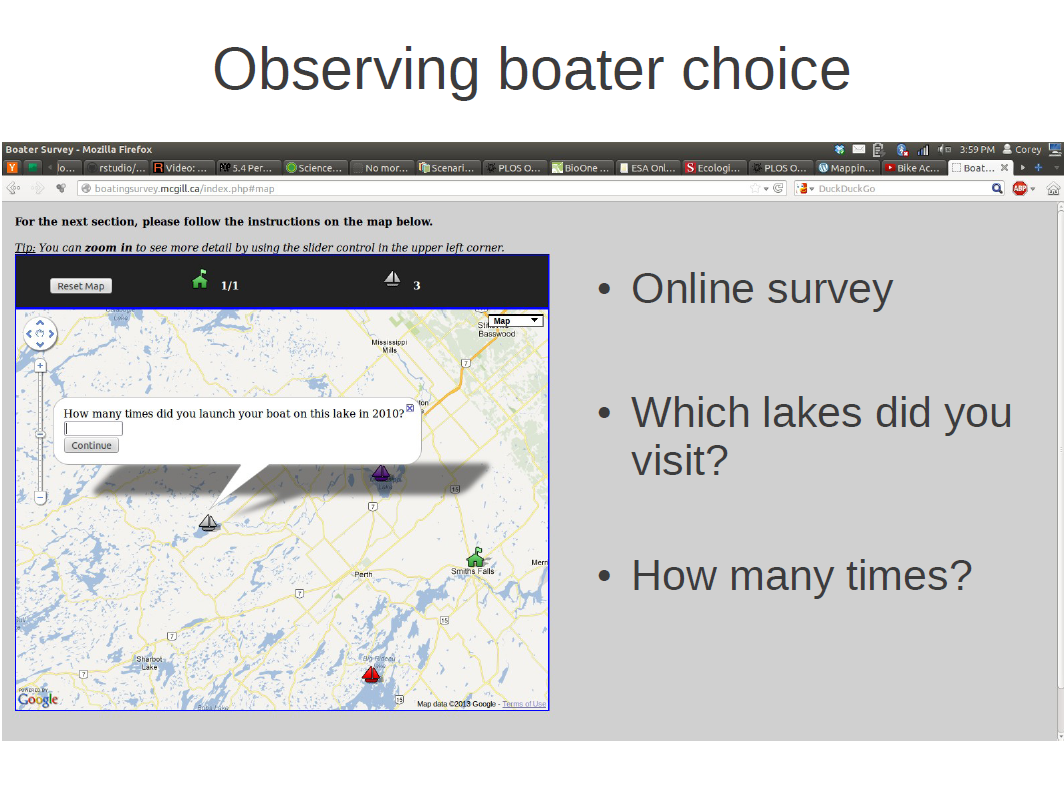
I wanted to observe boater choice in order to predict how propagules are likely flow between lakes. To do this I conducted an online survey. In the survey I asked boaters to identify which lakes they visited during the boating season, as well as how many times they visited each lake. Respondents were able to identify their responses on an interactive map, and were able to reminisce about all the great fish they caught that summer while they did it (they were doing it in December).

We ended up with 510 respondents with 146 boaters indicated that they visited multiple lakes.

In keeping with the methodology that I have outlined, I of course simulated some boaters making trip taking decisions in a simulated landscape. I had simulations with the boaters behaving according to each of the two behavioural models and in each simulation, I had those boater fill out a simulated survey just like the one I had online. By collecting this pseudo-data, I then went and looked at whether I could recapture the parameter values underlying the data.

Shown here are the results of that experiment, with the 1:1 line indicating perfect agreement between the actual and predicted values of each of the four parameters for each model. For the same set of simulations, I also checked to see whether I could correctly identify when the generating model was the gravity model, or the RUM.

So what where the results of the survey (the real, flesh and blood survey)?

Well, for the boaters I surveyed in Ontario, the gravity model functional form fit the observed data considerably better. This table just shows the delta AIC values for each of the models tested. Each value is relative to the best model with increasing values indicating decreasing fit.

Okay, so that’s maybe a mildly interesting. But it only matters insofar as whether it has an effect our prediction about spreading invasions. It turns out, that it does.

Because both models were fit using the same data and covariates, they both predicted the same amount of overall boater traffic between lakes, and hence the same net connectivity. The feature in which they differed, however, was in how that connectivity was distributed across the landscape.

We can measure this difference in connectivity distribution using a simple evenness measure like Shannon entropy. High entropy means a very even distribution, whereas low entropy means that the distribution of connectivity is more highly concentrated around few edges of the network. This connectivity distribution particularly matters when the spreading population experiences an Allee effect in its population dynamics. That is, when populations are disproportionately likely to go extinct at low population sizes, whether due to mate limitation in the case of sexually reproducing species, or other forms of density dependent growth. The reason this matters is that in dispersal networks with low entropy connectivity distributions, emigrants are not arriving in sufficient numbers to overcome the demographic barriers to establishment. There is a diluting effect in this situation. Whereas in low entropy connectivity networks, there are sufficient ‘hub’ patches, providing emigrants in sufficient numbers to overcome initial barriers to growth.

We can see this happening when we look at rates of spread in the GM and RUM cases. As Allee effects get stronger (going from left to right), the rates of spread in the early phases are much lower under the evenly distributed RUM dispersal network then under the more concentrated edge distribution of the gravity model.

While this is an important finding in the field of invasion dynamics, I think that this has implications more broadly and could be applied when looking at, instead of a population which we would like to suppress, a conservation setting where we are looking to preserve habitat patch connectivity.

But for now, back to populations which we are trying to suppress. I’ve shown so far how we can model the spread of aquatic invasives via their primary vector, which is recreational boaters. But ultimately, we want to know where they are likely to spread so that ideally, we can get out in front of them and actually do something about it.

One measure that has been proposed in some districts, is to place mandatory cleaning stations at strategically selected launch sites. The idea being to both prevent outgoing as well as incoming organisms to a lake. The problem, just like any lunch ever consumed in history, is that these are not free. There is a cost borne to the individual boaters, in the form of time. And there is cost associated with operating these stations, which may be passed on to boaters in the form of a mandatory usage fee.

The question becomes, then, how will boaters react in the face of such a cost, and how will their behaviours effect the efficacy of the policy?

To look at this question, I extended the original behavioral model to incorporate responses to management action. Boaters may choose a substitute lake to visit, redistributing their trips, or they may simply decided to stay home, reducing the total number of trips taken. Or they may do some combination of both. The observation model employs a binomial distribution of trip outcomes to estimate the behavioral parameters.

In order to estimate the behavioural responses, I conducting something that economists call ‘counterfactual’ analysis. This is a fancy word for ‘what if’ scenarios. After having identified which lakes they visited, I presented boaters with a hypothetical situation in which there were a mandatory cleaning procedure at one of the lakes which they indicated visiting. They were then asked how many times they would have used that lake, and how many times they would have used another lake which they had also identified visiting.

As always, using simulation I checked that my observation model was able to recapture the true parameters, given a sample of the same form and size as that which I would observe from the survey, with the expected amount of uncertainty around those estimates.

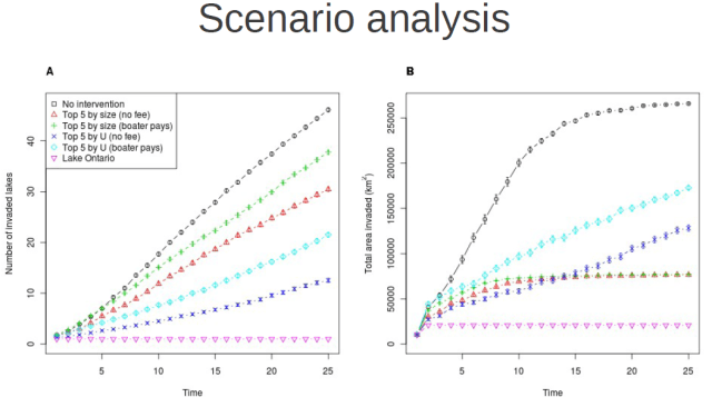
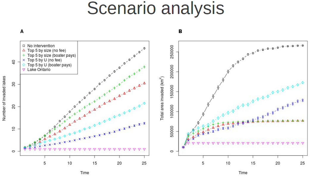
Once we have estimated the behavioural model parameters from the survey responses, we can start doing things like scenario analysis, wherein we impose any number of strategic interventions to see how the predicted rates of spread will respond.

So, I’ve outlined my case for how I think that we should approach ecological problems within the domain of management decisions, and I’ve given a few examples from my own work of this general methodology in action. Hopefully I’ve peeked your interest in this framework, and hopefully we’ll have lots to discuss, and potentially boisterously argue about over beers.