From Whale Calls to Dark Matter: Competitive Data Science with R and Python

Back in June I gave a fun talk at Montreal Python on some of my dabbling in the competitive data science scene. The good people at Savior-fair Linux recorded the talk and have edited it all together into a pretty slick video. If you can spare twenty-minutes or so, have a look.

If you want the slides, head on over to my speakerdeck page.

whaledarkmattercover

Advertisement

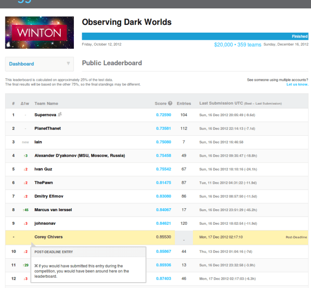
Dark matter top 10, but an hour too late

Well, that’s embarrassing. A little tweak to my dark matter model resulted in a leaderboard score in the top 10. The only problem is that the contest closed about an hour ago.

top_10

I ran this final prediction earlier today but then simply forgot to go back to it and submit!! On the bright side, I learned a lot of really interesting things about gravitational lensing and had a tonne of fun doing it. I’ll probably write a post-mortem sometime in the next few days, but for now I’m just kicking myself.

Simulating weak gravitational lensing

In the search for dark matter, I have been having mixed success. It seems that locating DM in single halo skies is a fairly straightforward problem. However, when there are more than one halo, things get quite a bit trickier.

As I have advocated many times before, including here and here, simulation can provide deep insights into many (if not all) problems. I never trust my own understanding of a complicated problem until I have simulated from a hypothesized model of that problem. Once I have a simulation in place, I can then test out all kinds of hypotheses about the system by manipulating the component parts. I think of this process as a kind of computer-assisted set of thought experiments.

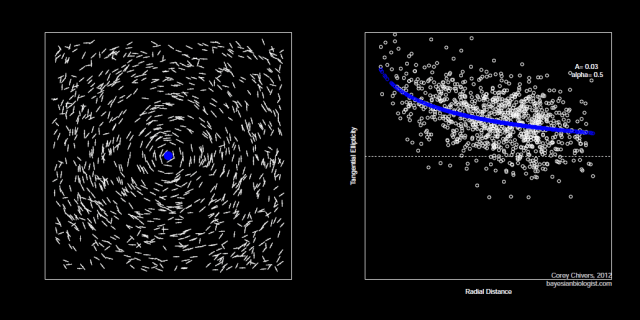
So, when I was hitting a wall with the dark matter challenge, I of course turned to simulation for insights. Normally this would have been my very first step, however in this case my level of understanding of the physics involved was insufficient when I started out. After having done a bit of reading on the topic, I built a model which implements a weak lensing regime on an otherwise random background of galaxies. The model assumes an Einasto profile of dark matter mass density, with parameters A and α determining the strength of the tangential shearing caused by foreground dark matter.

A=0.2, alpha=0.5

I can then increase the strength of the lens by either increasing the mass of the dark matter, or by varying the parameters of the Einasto profile.

A=0.059, alpha=0.5

A=0.03, alpha=0.5

You can check out this visualization over a range of A values.

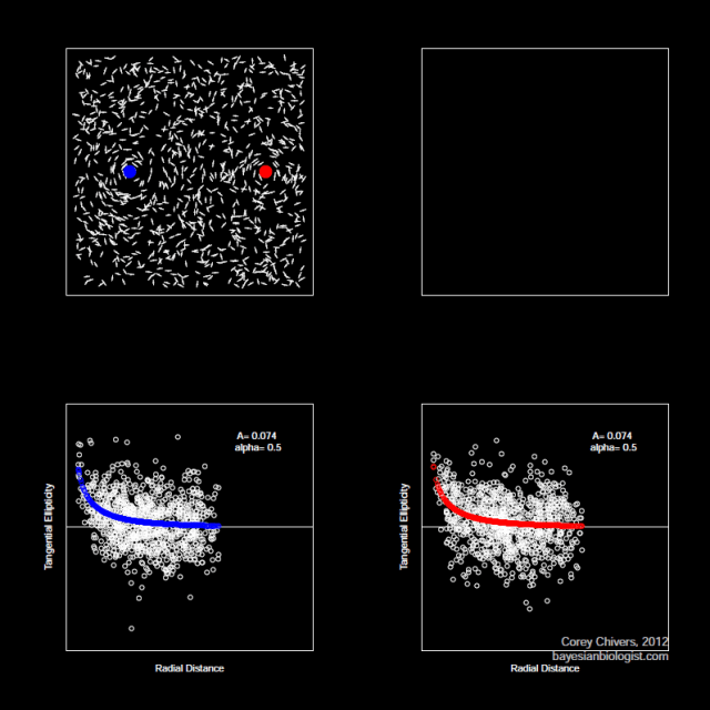
I can also see how two halos interact in terms of the induced tangential ellipticity profile by simulating two halos and then moving them closer to one another.

You can see the effect here. You get the idea – I can also try out any combination of configurations, shapes, and strengths of interacting halos. I can then analyse the characteristics of the resulting observable factors (in this case, galaxy location and ellipticities) in order to build better a predictive model.

Unfortunately, since this is a competition with cold hard cash on the line, I am not releasing the source for this simulation at this time. I will, however, open source the whole thing when the competition ends.

Dark matter benchmarks: All over the map

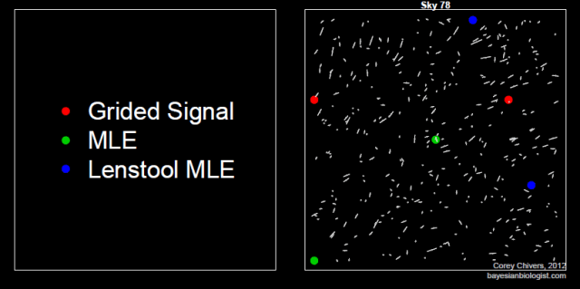
The three benchmark algorithms for predicting the location of dark matter halos are, for the most part, all over the map. Most of the test skies look something like this:

There are, however, some skies with rather strong halo signals that get a decent amount of agreement:

The Lenstool MLE algorithm is the current state of the art. As such, it’s the algo to beat. As of this morning, there was only one entry on the leader board with a score topping this benchmark.

*cracks fingers* – Let’s see if we can give it a run for it’s money.

Observing Dark Worlds – Visualizing dark matter’s distorting effect on galaxies

Some people like to do crossword puzzles. I like to do machine learning puzzles.

Lucky for me, a new contest was just posted yesterday on Kaggle. So naturally, my lazy Saturday was spent getting elbow deep into the data.

The training set consists of a series of ‘skies’, each containing a bunch of galaxies. Normally, these galaxies would exhibit random ellipticity. That is, if it weren’t for all that dark matter out there! The dark matter, while itself invisible (it is dark after all), tends to aggregate and do some pretty funky stuff. These aggregations of dark matter produce massive halos which bend the heck out of spacetime itself! The result is that any galaxies behind these halos (from our perspective here on earth) appear contorted around the halo.

The tricky bit is to distinguish between the background noise in the ellipticity of galaxies, and the regular effect of the dark matter halos. How hard could it be?

Step one, as always, is to have a look at what you’re working with using some visualization.

An example of the training data. This sky has 3 dark matter halos. I f you squint, you can kind of see the effect on the ellipticity of the surrounding galaxies.

If you want to try it yourself, I’ve posted the code here.

If you don’t feel like running it yourself, here are all 300 skies from the training set.


Now for the simple matter of the predictions. Looks like Sunday will be a fun day too! Stay tuned…

The essence of a handwritten digit

If you haven’t yet discovered the competitive machine learning site kaggle.com, please do so now. I’ll wait.

Great – so, you checked it out, fell in love and have made it back. I recently downloaded the data for the getting started competition. It consists of 42000 labelled images (28×28) of hand written digits 0-9. The competition is a straight forward supervised learning problem of OCR (Optical Character Recognition). There are two sample R scripts on the site to get you started. They implement the k-nearest neighbours and Random Forest algorithms.

I wanted to get  started by visualizing all of the training data by rendering some sort of an average of each character. Visualizing the data is a great first step to developing a model. Here’s how I did it:

## Read in data
train <- read.csv("../data/train.csv", header=TRUE)
train<-as.matrix(train)

##Color ramp def.
colors<-c('white','black')
cus_col<-colorRampPalette(colors=colors)

## Plot the average image of each digit
par(mfrow=c(4,3),pty='s',mar=c(1,1,1,1),xaxt='n',yaxt='n')
all_img<-array(dim=c(10,28*28))
for(di in 0:9)
{
print(di)
all_img[di+1,]<-apply(train[train[,1]==di,-1],2,sum)
all_img[di+1,]<-all_img[di+1,]/max(all_img[di+1,])*255

z<-array(all_img[di+1,],dim=c(28,28))
z<-z[,28:1] ##right side up
image(1:28,1:28,z,main=di,col=cus_col(256))
}

Which gives you:
Notice the wobbly looking ‘1’. You can see that there is some variance in the angle of the slant, with a tenancy toward leaning right. I imagine that this is due to the bias toward right handed individuals in the sample.

I also wanted to generate a pdf plot of all of the training set, to get myself an idea of what kind of anomalous instances I should expect.

If you are interested, dear reader, here is my code to do just that.

pdf('train_letters.pdf')
par(mfrow=c(4,4),pty='s',mar=c(3,3,3,3),xaxt='n',yaxt='n')
for(i in 1:nrow(train))
{
z<-array(train[i,-1],dim=c(28,28))
z<-z[,28:1] ##right side up
image(1:28,1:28,z,main=train[i,1],col=cus_col(256))
print(i)
}
dev.off()

Which will give you a 2625 page pdf of every character in the training set which you can, um, casually peruse.
As of the time of writing, the current leading submission has a classification accuracy of 99.27%. There is no cash for this competition, but the knowledge gained from taking a stab at it is priceless. So give it a shot!