This puzzle came up in the New York Times Number Play blog. It goes like this:
An entrepreneur has devised a gambling machine that chooses two independent random variables x and y that are uniformly and independently distributed between 0 and 100. He plans to tell any customer the value of x and to ask him whether y > x or x > y.
If the customer guesses correctly, he is given y dollars. If x = y, he’s given y/2 dollars. And if he’s wrong about which is larger, he’s given nothing.
The entrepreneur plans to charge his customers $40 for the privilege of playing the game. Would you play?
I figured I’d give it a go. Since I was feeling lazy, and already had my computer in front of me, I thought that I’d do it via simulation rather than working out the exact maths. I tried playing the game with the first strategy that came to mind. If x<50, I would choose y>x, and if x>50, I’d choose y<x, figuring I’d maximize my probability of winning something rather than nothing. This was probably due to the inherent risk aversion of system one. Let’s see how that works out:
N<-100000
x<-sample.int(100,N,replace=TRUE)
y<-sample.int(100,N,replace=TRUE)
dec_rule=50
payout<-numeric(N)
for(i in 1:N)
{
## Correct Guess (playing simple max p(!0) strategy)
if( (x[i]>dec_rule & y[i]<x[i]) | (x[i]<=dec_rule & y[i]>x[i]) )
payout[i]<-y[i]

## Incorrect Guess (playing simple max p(!0) strategy)
if( (x[i]>dec_rule & y[i]>x[i]) | (x[i]<=dec_rule & y[i]<x[i]) )
payout[i]<-0

## Tie pays out y/2
if(x[i] == y[i])
payout[i]<-y[i]/2
}
## Expected Payout ##
print(paste(dec_rule,mean(payout)))
Which leads to an expected payout of $37.75. Playing the risk averse strategy leads to an expected value less than the cost of admission, loosing on average 25 cents per play. No deal, Mr entrepreneur, I had something else in mind for my forty bucks anyway.
Lets try alternate strategies, and see if we can’t play in such a way as to improve our outlook.
## Gambling Machine Puzzle ##
## Puzzle presented in http://wordplay.blogs.nytimes.com/2013/03/04/machine/

result<-numeric(100)
for(dec_rule in 1:100)
{
N<-10000
x<-sample.int(100,N,replace=TRUE)
y<-sample.int(100,N,replace=TRUE)

payout<-numeric(N)

for(i in 1:N)
{
## Correct Guess (playing dec_rule strategy)
if( (x[i]>dec_rule & y[i]<x[i]) | (x[i]<=dec_rule & y[i]>x[i]) )
payout[i]<-y[i]

## Incorrect Guess (playing dec_rule strategy)
if( (x[i]>dec_rule & y[i]>x[i]) | (x[i]<=dec_rule & y[i]<x[i]) )
payout[i]<-0

## Tie pays out y/2
if(x[i] == y[i])
payout[i]<-y[i]/2
}

## Expected Payout ##
print(paste(dec_rule,mean(payout)))
result[dec_rule]<-mean(payout)
}
par(cex=1.5)
plot(result,xlab='Decision rule',ylab='E(payout)',pch=20)

abline(v=which.max(result))
abline(h=max(result))
abline(h=40,lty=3)
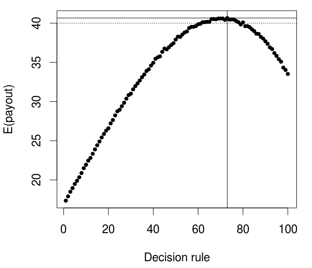
According to which, the best case scenario is an expected payout of $40.66, or an expected net of 66 cents per bet, if you were to play the strategy of choosing y>x for any x<73 and y<x for any x>73. You’re on, Mr entrepreneur!
To calculate the exactly optimal strategy and expected payout, we would need to compute the derivative of the expected payout function with respect to the within game decision threshold. I leave this fun stuff to the reader 😉


