What is probabilistic truth? Part 2 – Everything is conditional

Read Part 1

When making a statement of the form “1/2 is the correct probability that this coin will land tails”, there are a few things which are left unsaid, but which are typically implied.

The statement is one about the probability of an unknown event occurring, and it would seem reasonable to write this statement using probability notation as P(toss=tails) = 0.5. And indeed many people would express it this way. However, what is missing is the state of knowledge under which this statement has been made. For instance, is the coin yet to be flipped, or is it currently rolling in a circle on the table, leaning in toward its final resting position? Perhaps the flipping device can consistently throw a coin such that it rotates exactly 5 times in the air before landing flat on the table, or we know which side is up at the start of the flip. In these latter cases, the statement of probability would be made under considerably more knowledge than the first, and would not tend to be 0.5 in these cases. An observer placing a probability of P(toss=tails) = 0.99 at the moment when the coin is circling in on its resting position, leaning heavily toward a tails up configuration, could be said to have the correct probability also. For fairness, lets say that the first observer also makes her probability statement at the same moment, but from another room where she cannot see what has happened.

How can P(toss=tails) = 0.5, and P(toss=tails) = 0.99 be simultaneously correct?

The answer is conditioning. Each of the statements were made conditional on the observer’s state of knowledge. More completely, the two statements can be rewritten as:

P(toss=tails | knowledge of observer 1) = 0.5 , and

P(toss=tails | knowledge of observer 2) = 0.99

In practice, however, we often leave out the conditional part of the notation unless it is germane to the problem at hand. However, there is no such thing as unconditional probability. In fact, Harvard professor Joe Blitzstein calls conditioning the Soul of Statistics.

In the next post in this series, we’ll start looking at how to assess the correctness of a (conditional) probability statement after having observed an outcome.

Here's a bunch of random walks -- just 'cause its neat.

Here’s a bunch of random walks — just ’cause its neat.

Advertisement

Simulating Euro 2012

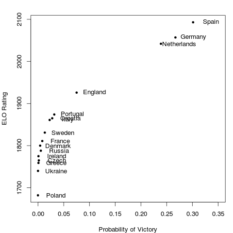
Why settle for just one realisation of this year’s UEFA Euro when you can let the tournament play out 10,000 times in silico?

Since I already had some code lying around from my submission to the Kaggle hosted 2010 Take on the Quants challenge, I figured I’d recycle it for the Euro this year. The model takes a simulation based approach, using Poisson distributed goals. The rate parameters in a given match are determined by the relative strength of each team as given by their ELO rating.

The advantage of this approach is that the tournament structure (which teams are assigned to which groups, how points are assigned, quarter final structure, etc) can be accounted for. If we wanted to take this into account when making probabilistic forecasts of tournament outcomes, we would need to calculate many conditional probability statements, following the extremely large number of possible outcomes. However, the downside is that it is only as reliable as the team ratings themselves. In my submission to Kaggle, I used a weighted average of ELO and FIFA ratings.

After simulating the tournament 10,000 times, the probability of victory for each team is just the number of times that team arose victorious divided by 10,000.

Feel free to get the code here and play around with it yourself. You can use your own rating system and see how the predicted outcomes change. If you are of a certain disposition, you might even find it more fun than the human version of the tournament itself!

Monty Hall by simulation in R

(Almost) every introductory course in probability introduces conditional probability using the famous Monte Hall problem. In a nutshell, the problem is one of deciding on a best strategy in a simple game. In the game, the contestant is asked to select one of three doors. Behind one of the doors is a great prize (free attendance to an R workshop, lets say), and there is a bum prize behind each of the other two doors. The bum prize is usually depicted to be a goat, but I don’t think that would be such a bad prize, so let’s say that behind two of the doors is a bunch of poorly collected data for you to analyse. Once the contestant makes her first selection, the host then opens one of the other two doors to reveal one of the bum prizes.

At this point, the contestant is given the choice to either stay with her original selection, or switch to the other remaining unopened door. What should she do?

If you’re reading this blog, you no doubt gleefully shouted “Switch! Switch! Daddy needs a ticket to that R workshop!”. And you also, no doubt, can prove this to be the best strategy using the logic of probability. You reason that the contestant’s chance of selecting the winning door from the onset was 1/3, giving her a 2/3 probability of being wrong. Once one door with a bum prize has been opened, the contestant is now choosing between two doors. Knowing that there was only a 1/3 chance that original selection was correct, there is now a 2/3 chance that the alternate door is the winner.

As I have mentioned in previous posts, I have found that engaging students to think through logical reasoning problems can be greatly enhanced by appealing to their desire to see it in action. To that end, I whipped up this little script to simulate repeatedly playing the Monte Hall game.


#####################################################
# Simulation of the Monty Hall Problem
# Demonstrates that switching gives you better odds
# than staying with your initial guess
#
# Corey Chivers, 2012
#####################################################

rm(list=ls())
monty<-function(strat='stay',N=1000,print_games=TRUE)
{
 doors<-1:3 #initialize the doors behind one of which is a good prize
 win<-0 #to keep track of number of wins

for(i in 1:N)
 {
 prize<-floor(runif(1,1,4)) #randomize which door has the good prize
 guess<-floor(runif(1,1,4)) #guess a door at random

## Reveal one of the doors you didn't pick which has a bum prize
 if(prize!=guess)
 reveal<-doors[-c(prize,guess)]
 else
 reveal<-sample(doors[-c(prize,guess)],1)

 ## Stay with your initial guess or switch
 if(strat=='switch')
 select<-doors[-c(reveal,guess)]
 if(strat=='stay')
 select<-guess
 if(strat=='random')
 select<-sample(doors[-reveal],1)

## Count up your wins
 if(select==prize)
 {
 win<-win+1
 outcome<-'Winner!'
 }else
 outcome<-'Losser!'

if(print_games)
 cat(paste('Guess: ',guess,
 '\nRevealed: ',reveal,
 '\nSelection: ',select,
 '\nPrize door: ',prize,
 '\n',outcome,'\n\n',sep=''))
 }
 cat(paste('Using the ',strat,' strategy, your win percentage was ',win/N*100,'%\n',sep='')) #Print the win percentage of your strategy
}

Students can then use the function to simulate N games under the strategies ‘stay’, ‘switch’, and ‘random’. Invoking the function using:


monty(strat="stay")
monty(strat="switch")
monty(strat="random")

Hey, look at that – it is better to switch! Feel free to use this in your own class, and let me know if you use it or adapt it in an interesting way!

Edit: Thanks to Ken for pointing out that saying that ‘switching is always better’ is not quite right (you will loose 1/3 of the time, after all), but rather that switching is a rational best strategy, given your state of knowledge.