Calculating AUC the hard way

The Area Under the Receiver Operator Curve is a commonly used metric of model performance in machine learning and many other binary classification/prediction problems. The idea is to generate a threshold independent measure of how well a model is able to distinguish between two possible outcomes. Threshold independent here just means that for any model which makes continuous predictions about binary outcomes, the conversion of the continuous predictions to binary requires making the choice of an arbitrary threshold above which will be a prediction of 1, below which will be 0.

AUC gets around this threshold problem by integrating across all possible thresholds. Typically, it is calculated by plotting the rate of false positives against false negatives across the range of possible thresholds (this is the Receiver Operator Curve)  and then integrating (calculating the area under the curve). The result is typically something like this:

auc

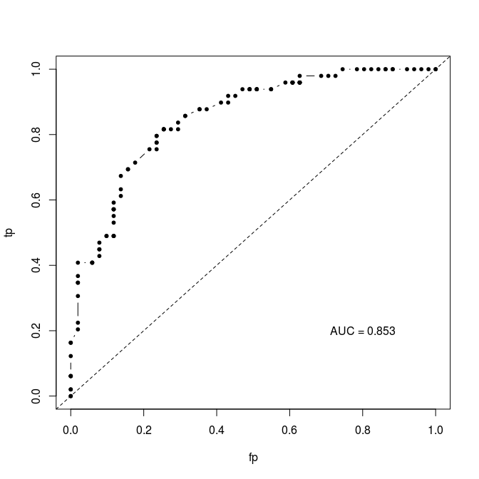
I’ve implemented this algorithm in an R script (https://gist.github.com/cjbayesian/6921118) which I use quite frequently. Whenever I am tasked with explaining the meaning of the AUC value however, I will usually just say that you want it to be 1 and that 0.5 is no better than random. This usually suffices, but if my interlocutor is of the particularly curious sort they will tend to want more. At which point I will offer the interpretation that the AUC gives you the probability that a randomly selected positive case (1) will be ranked higher in your predictions than a randomly selected negative case (0).

Which got me thinking – if this is true, why bother with all this false positive, false negative, ROC business in the first place? Why not just use Monte Carlo to estimate this probability directly?

So, of course, I did just that and by golly it works.

source("http://polaris.biol.mcgill.ca/AUC.R")
bs<-function(p)
{
 U<-runif(length(p),0,1)
 outcomes<-U<p
 return(outcomes)
}

# Simulate some binary outcomes #
n <- 100
x <- runif(n,-3,3)
p <- 1/(1+exp(-x))
y <- bs(p)

# Using my overly verbose code at https://gist.github.com/cjbayesian/6921118
AUC(d=y,pred=p,res=500,plot=TRUE)

## The hard way (but with fewer lines of code) ##
N <- 10000000
r_pos_p <- sample(p[y==1],N,replace=TRUE)
r_neg_p <- sample(p[y==0],N,replace=TRUE)

# Monte Carlo probability of a randomly drawn 1 having a higher score than
# a randomly drawn 0 (AUC by definition):

rAUC <- mean(r_pos_p > r_neg_p)
print(rAUC)

By randomly sampling positive and negative cases to see how often the positives have larger predicted probability than the negatives, the AUC can be calculated without the ROC or thresholds or anything. Now, before you object that this is necessarily an approximation, I’ll stop you right there – it is.  And it is more computationally expensive too. The real value for me in this method is for my understanding of the meaning of AUC. I hope that it has helped yours too!

Advertisement

Uncertainty matters

In a post I wrote earlier this year, I noted a sentiment expressed in The Economist about understanding and embracing uncertainty.

…recent reforms to the IPCC’s procedures will do little to change its tendency to focus on the areas where there is greater consensus, avoiding the uncertainties which, though unpalatable for scientists, are important to policy. (link)

Which I felt was contrary to the way we, as scientists, speak among ourselves about policy makers. Specifically, that it is they who fear and misunderstand the implications of uncertainty.

This is the same perception which has led to the launch today by the group Sense About Science of a publication titled Making Sense of Uncertainty: Why uncertainty is part of science.

Launching a guide to Making Sense of Uncertainty at the World Conference of Science Journalists today, researchers working in some of the most significant, cutting edge fields say that if policy makers and the public are discouraged by the existence of uncertainty, we miss out on important discussions about the development of new drugs, taking action to mitigate the impact of natural hazards, how to respond to the changing climate and to pandemic threats.

Interrogated with the question ‘But are you certain?’, they say, they have ended up sounding defensive or as though their results are not meaningful. Instead we need to embrace uncertainty, especially when trying to understand more about complex systems, and ask about operational knowledge: ‘What do we need to know to make a decision? And do we know it?’

The report seems to be in line with arguments I have made about uncertainty and decision making as they pertain to ecological research, management, and policy.

Among the contributors to the report is someone who I consider to be among the best when it comes to understanding and communicating uncertainty, David Spiegelhalter. While I haven’t made my way all the way through it yet, it looks like this report will be an informative read for both scientists and policy makers (oh ya, and journalists — can’t forget about them).

Who knows, we might be able to stop the finger pointing and work together in mutual understanding of the importance of uncertainty.

How likely is the NSA PRISM program to catch a terrorist?

Recent revelations about PRISM, the NSA’s massive program of surveillance of civilian communications have caused quite a stir. And rightfully so, as it appears that the agency has been granted warrantless direct access to just about any form of digital communication engaged in by American citizens, and that their access to such data has been growing significantly over the past few years.

Some may argue that there is a necessary trade-off between civil liberties and public safety, and that others should just quit their whining. Lets take a look at this proposition (not the whining part). Specifically, let’s ask: how much benefit, in terms of thwarted would-be attacks, does this level of surveillance confer?

Lets start by recognizing that terrorism is extremely rare. So the probability that an individual under surveillance (and now everyone is under surveillance) is also a terrorist is also extremely low. Lets also assume that the neck-beards at the NSA are fairly clever, if exceptionally creepy. We assume that they have devised an algorithm that can detect ‘terrorist communications’ (as opposed to, for instance, pizza orders) with 99% accuracy.

P(+ |  bad guy) = 0.99

A job well done, and Murica lives to fight another day. Well, not quite. What we really want to know is: what is the probability that they’ve found a bad guy, given that they’ve gotten a hit on their screen? Or,

P(bad guy | +) =??

Which is quite a different question altogether. To figure this out, we need a bit more information. Recall that bad guys (specifically terrorists) are extremely rare, say on the order of one in a million (this is a wild over estimate with the true rate being much lower, of course – but lets not let that stop us). So,

P(bad guy) = 1/1,000,000

Further, lets say that the spooks have a pretty good algorithm that only comes up falsely positive (ie when the person under surveillance is a good guy) one in one hundred times.

P(+ |  good guy) = 0.01

And now we have all that we need. Apply a little special Bayes sauce:

P(bad guy | +) = P(+ | bad guy) P(bad guy)  /  [ P(+ |  bad guy) P(bad guy) + P(+ |  good guy) P(good guy) ]

and we get:

P(bad guy | +) = 1/10,102

That is, for every positive (the NSA calls these ‘reports’) there is only a 1 in 10,102 chance (using our rough assumptions) that they’ve found a real bad guy.

UPDATE: While former NSA analyst turned whistle blower William Binney thinks this is a plausible estimate, the point here is not that this is the ‘correct probability‘ involved (remember that we based our calculations on very rough assumptions). The take away message is simply that whenever the rate of an event of interest is extremely low, even a very accurate test will fail very often.

UPDATE 2: The Wall Street Journal’s Numbers Guy has written a piece on this in which several statisticians and security experts respond.

UPDATE 3: If you can read German, a reader reached me to point out that Der Spiegel technology section picked up the story.

Big brother is always watching, but he’s still got a needle in a haystack problem.

Big Brother 11

The television series doesn’t have this problem. On the show, they’re all bad guys.

What is probabilistic truth? Part 2 – Everything is conditional

Read Part 1

When making a statement of the form “1/2 is the correct probability that this coin will land tails”, there are a few things which are left unsaid, but which are typically implied.

The statement is one about the probability of an unknown event occurring, and it would seem reasonable to write this statement using probability notation as P(toss=tails) = 0.5. And indeed many people would express it this way. However, what is missing is the state of knowledge under which this statement has been made. For instance, is the coin yet to be flipped, or is it currently rolling in a circle on the table, leaning in toward its final resting position? Perhaps the flipping device can consistently throw a coin such that it rotates exactly 5 times in the air before landing flat on the table, or we know which side is up at the start of the flip. In these latter cases, the statement of probability would be made under considerably more knowledge than the first, and would not tend to be 0.5 in these cases. An observer placing a probability of P(toss=tails) = 0.99 at the moment when the coin is circling in on its resting position, leaning heavily toward a tails up configuration, could be said to have the correct probability also. For fairness, lets say that the first observer also makes her probability statement at the same moment, but from another room where she cannot see what has happened.

How can P(toss=tails) = 0.5, and P(toss=tails) = 0.99 be simultaneously correct?

The answer is conditioning. Each of the statements were made conditional on the observer’s state of knowledge. More completely, the two statements can be rewritten as:

P(toss=tails | knowledge of observer 1) = 0.5 , and

P(toss=tails | knowledge of observer 2) = 0.99

In practice, however, we often leave out the conditional part of the notation unless it is germane to the problem at hand. However, there is no such thing as unconditional probability. In fact, Harvard professor Joe Blitzstein calls conditioning the Soul of Statistics.

In the next post in this series, we’ll start looking at how to assess the correctness of a (conditional) probability statement after having observed an outcome.

Here's a bunch of random walks -- just 'cause its neat.

Here’s a bunch of random walks — just ’cause its neat.

What is probabilistic truth?

I am currently working on a validation metric for binary prediction models. That is, models which make predictions about outcomes that can take on either of two possible states (eg Dead/not dead, heads/tails, cat in picture/no cat in picture, etc.) The most commonly used metric for this class of models is AUC, which assesses the relative error rates (false positive, false negative) across the whole range of possible decision thresholds. The result is a curve that looks something like this:

auc

Where the area under the curve (the curve itself is the Receiver Operator Curve (ROC)) is some value between 0 and 1. The higher this value, the better your model is said to perform. The problem with this metric, as many authors have pointed out, is that a model can perform very well in terms of AUC, but be completely miscalibrated in terms of the actual probabilities placed on each outcome.

A model which distinguishes perfectly between positive and negative cases (AUC=1) by placing a probability of 0.01 on positive cases and 0.001 on negative cases may be very far off in terms of the actual probability of a positive case. For instance, positive cases may actually occur with probability 0.6 and negative cases with 0.2. In most real situations, our models will predict a whole range of different probabilities with a unique prediction for each data point, but the general idea remains. If your goal is simply to distinguish between cases, you may not care whether the probabilities are not correct. However, if your model is purporting to quantify risk then you very much want to know if you are placing the probabilistically true predictions on cases that are yet to be observed.

Which begs the question: What is probabilistic truth? 

This questions appears, at least at first, to be rather simple. A frequentist definition would say that the probability is correct, or true, if the predicted probability is equal to the long run outcomes.  Think of a dice rolled over and over counting the number of times a one is rolled. We would compare this frequency to our predicted probability of rolling a one (1/6 for a fair six-sided die) and would say that our predicted probability was true if this frequency matched 1/6.

But what about situations where we can’t re-run an experiment over and over again? How then would we evaluate the probabilistic truth of our predictions?

I’ll be working through this problem in a series of posts in the coming weeks. Stay tuned!

Read Part 2

Mathematical abstraction and the robustness to assumptions

I’ve been showing my new favourite toys to just about anyone foolish enough to actually engage me in conversation. I described how my shiny new set of non-transitive dice work here, complete with a map showing all the relevant probabilities.

All was neat and tidy and wonderful until fellow ecologist, Aaron Ball, tried to burst my bubble.

Nope. I couldn’t find the error. Fortunately, he works across the hall so I just went and asked him.

The problem he found, it turns out, was not with my calculations but with my assumptions. Aaron told me that dice constructed with rounded corners and hollowed out pips for the numbers on the faces tend to be biased in the frequency at which each face rolls up. I had assumed, of course, that each side of each of the five dice would roll with the same probability (ie. 1 in 6).

As with any model of a real world system, the mathematics were carried out on a simplified abstraction of the system being modelled. There are always, by necessity, assumptions being made. The important thing is to make these assumptions as explicit as possible and, where possible, to test the robustness of the model predictions to violations of the assumptions. Implicit to my calculations of the odds of the non-transitive Grime dice was the assumption that the dice are fair.

To check the model for robustness to this assumption, we can relax it and find out if we still get the same behaviour. Specifically, we can ask here whether some sort of pip-and-rounded-corner-induced bias can lead to a change in the Grime dice non-transitive cycles.

It seems a natural place to look would be between the dice pairings which have the closest to even odds. We can find out what level of bias would be required to switch the directionality of the odds (or at least erase the tendency for one die to roll higher than the other). Lets try looking at Magenta and Red, which under the fair dice assumption have odds p(Magenta > Red)=5/9. What kind of bias will change this relationship? The odds can be evened out by either Magenta rolling ones more often, or red rolling nine more often. The question is then, how much bias would there need to in the dice in order to even out the odds between Magenta and Red?

Lets start with Red biasing toward rolling nine more often (recall that nine appears on only one face). Under the fair dice hypothesis, Red can roll nine (1/6 of the time) and win no matter what Magenta rolls, or by rolling four (5/6 of the time) and win when Magenta rolls one (1/3 of the time).

P(Red > Magenta) = 1/6 + 5/6 * 1/3, which is 4/9.

If we set this probability equal to 1/2, and replace the fraction of times that Red rolls nine with x, we can solve for the frequency needed to even the odds.

x + 5/6 * 1/3 = 1/2

x = 2/9

Meaning that the Red die would have to be biased toward rolling nine with 2/9 odds. That’s equivalent to rolling a nine 1 and 1/3 times (33%) more often than you would expect if the die were fair!

Alternatively, the other way the odds between Red and Magenta could be evened is if Magenta biased towards rolling ones more often. We can do the same kind of calculation as above to figure out how much bias would be needed.

1/6 + 5/6 * x = 1/2

x = 2/5

Which corresponds to Magenta having  a 20% bias toward rolling ones. Of course, some combination of these biases could also be possible.

I leave it to the reader to work out the other pairings, but from the Red-Magenta analysis we can see that even if the dice deviated quite a bit from the expected 1/6 probability for each side, the edge afforded to Magenta is retained. I couldn’t find any convincing  evidence for the extent of bias caused by pipping and rounded corners but it seems unlikely that it would be strong enough to change the structure of the game.

A quick guide to non-transitive Grime Dice

A very special package that I am rather excited about arrived in the mail recently. The package contained a set of 6-sided dice. These dice, however, don’t have the standard numbers one to six on their faces. Instead, they have assorted numbers between zero and nine. Here’s the exact configuration:

red<-c(4,4,4,4,4,9)
blue<-c(2,2,2,7,7,7)
olive<-c(0,5,5,5,5,5)
yellow<-c(3,3,3,3,8,8)
magenta<-c(1,1,6,6,6,6)

Aside from maybe making for a more interesting version of snakes and ladders, why the heck am I so excited about these wacky dice? To find out what makes them so interesting, lets start by just rolling one against another and seeing which one rolls the higher number. Simple enough. Lets roll Red against Blue. Until you get your own set, you can roll in silico.

That was fun. We can do it over and over again and we’ll find that Red beats Blue more often than not. So it seems like Red is a pretty good bet. Now lets try rolling Olive against Red. I’ll wait.

Hey, look at that, the mighty Red has fallen. Olive tends to roll a higher number than Red more often than it doesn’t. So far, we have discovered this relationship:

Olive > Red > Blue

All hail the dominant Olive! Out of these three dice, if we want the best chance of winning, we should always pick Olive right? No dice, as they say. When we roll Olive against Blue, we find that Blue wins more often!

For any one of these three dice, there is another that will roll a higher number more often than not.

Olive > Red > Blue > Olive > Red > Blue > Olive > Red > Blue..

This forms a chain of dominance relationships that is a closed cycle. This property is called intransivity, and you can use it to win riches beyond your wildest dreams, er, well, at least to impress your friends.

Neat, right? But there’s more! We can do the same trick with Yellow, Magenta, and Red (Red > Magenta > Yellow > Red > …). With all five dice, there is a chain for which the order is given by that length of the word for each colour.

Red > Blue > Olive > Yellow > Magenta > …

Awesome. But that’s not it, either! You may have noticed from our three way comparisons that there is another five way chain. This time, the chain order is given by the alphabetical order of the words for each of the colours.

Blue > Magenta > Olive > Red > Yellow > …

What are the odds?

So far I’ve just asked you to take my word for it that the dominance relationships are as I described. Working out the odds of winning for any given pairing of dice as actually quite straightforward. Start by looking at the number on each side of the first die, one at a time. Count how many sides on the opposing die are less than the current number and divide by six. Since each side on the first die has a 1/6 chance of appearing, divide by 6 again. Sum these values for all six sides and you will have the probability that the first die will roll a higher number than the second.

For example, P(Red > Blue) = 5/6 x 1/2 + 1/6, which is 7/12.

Here I’ve worked out all of the pairwise odds:

Grime_dice

So, you can always win in this game as long as you get to be second to choose a colour. The odds are strongest in your favour when your opponent either chooses Magenta or Red, and you choose Olive or Yellow, respectively. Isn’t probability wonderful!

And if you still want more, it turns out that if you roll the Grime dice in pairs, the order of the word length chain reverses!

As a follow up to my simulation based approximate solution to the Gambling Machine Puzzle, here is the exact solution from mathematician Michael Lugo with a nice explaination.

God plays dice

From the New York Times “Numberplay” blog:

An entrepreneur has devised a gambling machine that chooses two independent random variables x and y that are uniformly and independently distributed between 0 and 100. He plans to tell any customer the value of x and to ask him whether y > x or x > y.

If the customer guesses correctly, he is given y dollars. If x = y, he’s given y/2 dollars. And if he’s wrong about which is larger, he’s given nothing.

The entrepreneur plans to charge his customers $40 for the privilege of playing the game. Would you play?

Clearly the strategy is to guess that y > x if x is small, and to guess that y < x if x is large. Say you’re told x = 60. If you guess x is the larger variable, then conditional on your guess being correct (which…

View original post 459 more words

The Gambling Machine Puzzle

This puzzle came up in the New York Times Number Play blog. It goes like this:

An entrepreneur has devised a gambling machine that chooses two independent random variables x and y that are uniformly and independently distributed between 0 and 100. He plans to tell any customer the value of x and to ask him whether y > x or x > y.

If the customer guesses correctly, he is given y dollars. If x = y, he’s given y/2 dollars. And if he’s wrong about which is larger, he’s given nothing.

The entrepreneur plans to charge his customers $40 for the privilege of playing the game. Would you play?

I figured I’d give it a go.  Since I was feeling lazy, and already had my computer in front of me, I thought that I’d do it via simulation rather than working out the exact maths. I tried playing the game with the first strategy that came to mind. If x<50, I would choose y>x, and if x>50, I’d choose y<x, figuring I’d maximize my probability of winning something rather than nothing. This was probably due to the inherent risk aversion of system one. Let’s see how that works out:

N<-100000
x<-sample.int(100,N,replace=TRUE)
y<-sample.int(100,N,replace=TRUE)
dec_rule=50
payout<-numeric(N)
for(i in 1:N)
{
## Correct Guess (playing simple max p(!0) strategy)
if( (x[i]>dec_rule & y[i]<x[i]) | (x[i]<=dec_rule & y[i]>x[i]) )
payout[i]<-y[i]

## Incorrect Guess (playing simple max p(!0) strategy)
if( (x[i]>dec_rule & y[i]>x[i]) | (x[i]<=dec_rule & y[i]<x[i]) )
payout[i]<-0

## Tie pays out y/2
if(x[i] == y[i])
payout[i]<-y[i]/2
}
## Expected Payout ##
print(paste(dec_rule,mean(payout)))

Which leads to an expected payout of $37.75. Playing the risk averse strategy leads to an expected value less than the cost of admission, loosing on average 25 cents per play. No deal, Mr entrepreneur, I had something else in mind for my forty bucks anyway.

Lets try alternate strategies, and see if we can’t play in such a way as to improve our outlook.

## Gambling Machine Puzzle ##
## Puzzle presented in http://wordplay.blogs.nytimes.com/2013/03/04/machine/

result<-numeric(100)
for(dec_rule in 1:100)
{
N<-10000
x<-sample.int(100,N,replace=TRUE)
y<-sample.int(100,N,replace=TRUE)

payout<-numeric(N)

for(i in 1:N)
{
## Correct Guess (playing dec_rule strategy)
if( (x[i]>dec_rule & y[i]<x[i]) | (x[i]<=dec_rule & y[i]>x[i]) )
payout[i]<-y[i]

## Incorrect Guess (playing dec_rule strategy)
if( (x[i]>dec_rule & y[i]>x[i]) | (x[i]<=dec_rule & y[i]<x[i]) )
payout[i]<-0

## Tie pays out y/2
if(x[i] == y[i])
payout[i]<-y[i]/2
}

## Expected Payout ##
print(paste(dec_rule,mean(payout)))
result[dec_rule]<-mean(payout)
}
par(cex=1.5)
plot(result,xlab='Decision rule',ylab='E(payout)',pch=20)

abline(v=which.max(result))
abline(h=max(result))
abline(h=40,lty=3)

gmachine

According to which, the best case scenario is an expected payout of $40.66, or an expected net of 66 cents per bet, if you were to play the strategy of choosing y>x for any x<73 and y<x for any x>73. You’re on, Mr entrepreneur!

To calculate the exactly optimal strategy and expected payout, we would need to compute the derivative of the expected payout function with respect to the within game decision threshold. I leave this fun stuff to the reader 😉

The Professor, the Bikini Model and the 5 Sigma Mistake

Today in The New York Times Magazine Maxine Swann tells the curious story of Paul Frampton, a 68 year old theoretical particle physicist who was apparently duped into becoming a drug mule by a bikini model he met online. The story is a fascinating tale of a giant academic ego and the seemingly infinite gullibility of this scientist.

Something stood out in particular for me. During the trial, Frampton was asked about several notes and calculations that were found on him when he was arrested. He had jotted: “5 standard deviations 99.99994%”, which he explained in court to be the criterion for the discovery of the Higgs Boson; a result that is unlikely to occur due to chance. He further explained that he was “calculating the probability that Denise Milani would become my second wife, which was almost a certainty.” Apparently, he took the messages and love notes that he had exchanged online with the purported ‘Milani’ to be strong evidence that she loved him. Under the null hypothesis — she doesn’t love me — these behaviours would have been very unlikely indeed.

Aside from committing the p-value fallacy, what else is wrong with Frampton’s logic?

The fact that Frampton was being set up was immediately obvious to his friend, who warned him about what was up in no uncertain terms. Most of us would have taken all the information available to us to make a conclusion. How often do young bikini models fall for older professors with a poor relationship track record, for instance? However, Frampton choose to only use a select set of observations on which to make his inference. Had he have incorporated prior information, or updated his beliefs as new evidence became available, he may have been able to avoid his 5 sigma mistake, and the nearly 5 years of jail time which he was sentenced for it.