Montreal R Workshop: Likelihood Methods and Model Selection

Monday, March 19, 2012  14h-16h, Stewart Biology N4/17

Corey Chivers, McGill University Department of Biology

This workshop will introduce participants to the likelihood principal and its utility in statistical inference.  By learning how to formalize models through their likelihood function, participants will learn how to confront these models with data in order to make statistical inference.

The concepts of using maximum likelihood to fit model parameters, and model comparison using information theoretic approaches will also be covered.

The workshop will explore these topics through worked examples and exercises using the R statistical computing environment.

This is the first official meetup of the Montreal R User Group. Be sure to join the group and RSVP. More information about the workshop here.

New R User Group in Montreal

The Montreal R User Group is now official. You can join the group by visiting the meetup site.


The group has existed since 2010 in a narrower incarnation as the BGSA R/Stats Workshop Series. Previous workshops have featured invited facilitators on topics such as Causal Analysis, GLMs, GAMs, Multi-model inference, Phylogenetic analysis, Bayesian modeling, Meta-analysis, Ordination, Programming and more. Our goal is to broaden the scope of the workshops to incorporate topics from a wide variety of applied fields.

We are kicking off with a meetup on Monday, March 19th. At the meeting, I will be facilitating a workshop on building and estimating Maximum Likelihood models and doing model selection using AIC.

We look forward to seeing you at the next meetup!

Montreal R User Group Organizers
Corey Chivers
Etienne Low-Décarie
Zofia Ecaterina Taranu
Eric Pedersen

π Day Special! Estimating π using Monte Carlo

In honour of π day (03.14 – can’t wait until 2015~) , I thought I’d share this little script I wrote a while back for an introductory lesson I gave on using Monte Carlo methods for integration.

The concept is simple – we can estimate the area of an object which is inside another object of known area by drawing many points at random in the larger area and counting how many of those land inside the smaller one. The ratio of this count to the total number of points drawn will approximate the ratio of the areas as the number of points grows large.

If we do this with a unit circle inside of a unit square, we can re-arrange our area estimate to yield an estimate of  π!

This R script lets us see this Monte Carlo routine in action:

##############################################
### Monte Carlo Simulation estimation of pi ##
## Author: Corey Chivers                    ##
##############################################

rm(list=ls())

options(digits=4)

## initialize ##
N=500 # Number of MC points
points <- data.frame(x=numeric(N),y=numeric(N))
pi_est <- numeric(N)
inner <-0
outer <-0

## BUILD Circle ##
circle <- data.frame(x=1:360,y=1:360)

for(i in 1:360)
{
circle$x[i] <-0.5+cos(i/180*pi)*0.5
circle$y[i] <-0.5+sin(i/180*pi)*0.5
}

## SIMULATE ##
pdf('MCpiT.pdf')

layout(matrix(c(2,3,1,1), 2, 2, byrow = TRUE))
for(i in 1:N)
{

# Draw a new point at random
points$x[i] <-runif(1)
points$y[i] <-runif(1)

# Check if the point is inside
# the circle
if( (points$x[i]-0.5)^2 + (points$y[i]-0.5)^2 > 0.25 )
{
outer=outer+1
}else
{
inner=inner+1
}

current_pi<-(inner/(outer+inner))/(0.25)
pi_est[i]= current_pi
print(current_pi)

par(mar = c(5, 4, 4, 2),pty='m')
plot(pi_est[1:i],type='l',
main=i,col="blue",ylim=c(0,5),
lwd=2,xlab="# of points drawn",ylab="estimate")
# Draw true pi for reference
abline(pi,0,col="red",lwd=2)

par(mar = c(1, 4, 4, 1),pty='s')
plot(points$x[1:i],points$y[1:i],
col="red",
main=c('Estimate of pi: ',formatC(current_pi, digits=4, format="g", flag="#")),
cex=0.5,pch=19,ylab='',xlab='',xlim=c(0,1),ylim=c(0,1))
lines(circle$x,circle$y,lw=4,col="blue")
frame() #blank

}
dev.off()
##############################################
##############################################

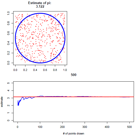
The resulting plot (multi-page pdf) lets us watch the estimate of π converge toward the true value.

At 500 sample points, I got an estimate of 3.122 – not super great. If you want to give your computer a workout, you can ramp up the number of iterations (N) and see how close your estimate can get. It should be noted that this is not an efficient way of estimating π, but rather a nice and simple example of how Monte Carlo can be used for integration.

In the lesson, before showing the simulation, I started by having students pair up and manually draw points, plot them, and calculate their own estimate.

If you use this in your classroom, drop me a note and let me know how it went!

Montreal R workshop: Plyr, reshape and other data manipulation goodies

March 12, 2012 14h-16h N4/17 Stewart Biology Building, McGill University

Étienne Low-Decarie, McGill University


This workshop is organized by the BGSA and is free of charge (!), but space is limited. Register early to ensure your spot!

From Étienne:

  • Ever want to split your data according to factors, apply a function on each part and combine all the results into a consistent output?
  • Want a table of the slope for each year of your sampling data?
  • Want a plot for each level of your treatment?
  • Want to transform your data (e.g.: standardization)?
  • And want the high speed benefits of parallelization to boot?!

If yes, come out the the workshop!

Visualising the Metropolis-Hastings algorithm

In a previous post, I demonstrated how to use my R package MHadapive to do general MCMC to estimate Bayesian models. The functions in this package are an implementation of  the Metropolis-Hastings algorithm. In this post, I want to provide an intuitive way to picture what is going on ‘under the hood’ in this algorithm.

The main idea is to draw samples from a distribution which you can evaluate at any point, but not necessarily  integrate (or at least, you don’t want to). The reason that integration is important come from Bayes theorem itself:

P(θ|D)=P(D|θ)P(θ)/P(D)

Where P(D) is the unconditional probability of observing the data. Since this is not dependant on the parameters of the model (θ) on which we wish to perform inference, P(D) is effectively a normalising constant which makes P(θ|D) a proper probability density function (ie. integrates to 1).

So, we have a non-normalised probability density function which we wish to estimate by taking random samples. The process of taking random samples itself is often difficult for complex models, so instead we explore the distribution using a Markov chain. We need a chain which, if run long enough, will consist as a whole of random samples from our distribution of interest (lets call that distribution π). This property of the Markov chain we are constructing is called ergodicity. The Metropolis-Hastings algorithm is a way to construct such a chain.

It works like this:

  1. Choose some starting point in the parameter space k_X
  2. Choose a candidate point k_Y ~ N(k_X, σ). This is often referred to as the proposal distribution.
  3. Move to the candidate point with probability:  min( π(k_Y)/π(K_X), 1)
  4. Repeat.

The following code demonstrates this process in action for a simple normal target distribution.

################################################################
###     Metropolis-Hastings Visualization                #######
###      Created by Corey Chivers, 2012                #########
################################################################

mh_vis<-function(prop_sd=0.1,target_mu=0,
target_sd=1,seed=1,iter=5000,plot_file='MH.pdf')
{
plot_range=c(target_mu-3*target_sd,target_mu+3*target_sd)
track <- NULL
k_X = seed; ## set k_X to the seed position

pdf(plot_file)
par(mfrow=c(3,1),mgp = c(1, 0.5, 0))

for(i in 1:iter)
{
track<-c(track,k_X)    ## The chain
k_Y = rnorm(1,k_X,prop_sd) ## Candidate point

## -- plot kernal density estimation of the Chain
par(mar=c(0,3,2,3),xaxt='n',yaxt='n')

curve(dnorm(x,target_mu,target_sd),col='blue',lty=2,lwd=2,xlim=plot_range)
if(i > 2)
lines(density(track,adjust=1.5),col='red',lwd=2)

## -- plot the chain
par(mar=c(0,3,0,3))
plot(track,1:i,xlim=plot_range,main='',type='l',ylab='Trace')

pi_Y = dnorm(k_Y,target_mu,target_sd,log=TRUE)
pi_X = dnorm(k_X,target_mu,target_sd,log=TRUE)

## -- plot the target distribution and propsal distribution actions
par(mar=c(3,3,0,3),xaxt='s')
curve(dnorm(x,target_mu,target_sd),xlim=plot_range,col='blue',lty=2,ylab='Metropolis-Hastings',lwd=2)
curve(dnorm(x,k_X,prop_sd),col='black',add=TRUE)
abline(v=k_X,lwd=2)
points(k_Y,0,pch=19,cex=2)
abline(v=k_Y)

a_X_Y = (pi_Y)-(pi_X)
a_X_Y = a_X_Y

if (a_X_Y > 0)
a_X_Y = 0

## Accept move with a probability a_X_Y
if (log(runif(1))<=a_X_Y)
{
k_X = k_Y;
points(k_Y,0,pch=19,col='green',cex=2)
abline( v=k_X,col='black',lwd=2)
}
## Adapt the poposal
if(i>100)
prop_sd=sd(track[floor(i/2):i])

if(i%%100==0)
print(paste(i,'of',iter))
}
dev.off()
}

mh_vis()

A common problem in the implementation of this algorithm is the selection of σ. Efficient mixing (the rate at which the chain converges to the  target distribution) occurs when σ approximates the standard deviation of the target distribution. When we don’t know this value in advance. we can allow σ to adapt based on the history of the chain so far. In the above example, σ is simply updated to take the value of the standard deviation of some previous points in the chain.

The output is a multipage pdf which you can scroll through to animate the MCMC.

The top panel shows the target distribution (blue dotted) and a kernel smoothed estimate of the target via the MCMC samples. The second panel shows a trace of the chain, and the bottom panel illustrates the steps of the algorithm itself.

Note: notice the first 100 or so iterations were a rather poor representation of the target distribution. In practice, we would ‘burn’ the first n iterations of the chain – typically the first 100-1000.

Gauging Interest in a Montreal R User Group

** UPDATE ** We’ve done it! Visit the Montreal R User Group site to join.

Some of us over at McGill’s Biology Graduate Student Association have been developing and delivering R/Statistics workshops over the last few years. Through invited graduate students and faculty, we have tackled  everything from multi-part introductory workshops to get your feet wet, to special topics such as GLMs, GAMs, Multi-model inference, Phylogenetic analysis, Bayesian modeling, Meta-analysis, Ordination, Programming and more.

We are currently toying with the idea of opening the workshop beyond the department, and even beyond McGill by founding a Montreal R User Group. If you are interested in attending and/or speaking at a Montreal R User Group, we’d love to hear from you! If there is enough interest, we’ll start up a group.

General Bayesian estimation using MHadaptive

If you can write the likelihood function for your model, MHadaptive will take care of the rest (ie. all that MCMC business). I wrote this R package to simplify the estimation of posterior distributions of arbitrary models. Here’s how it works:

1) Define your model (ie the likelihood * prior). In this example, lets build a simple linear regression model.

(log)Likelihood:

li_reg<-function(pars,data)
{
a<-pars[1]      #intercept
b<-pars[2]      #slope
sd_e<-pars[3]   #error (residuals)
if(sd_e<=0){return(NaN)}
pred <- a + b * data[,1]
log_likelihood<-sum( dnorm(data[,2],pred,sd_e, log=TRUE) )
prior<- prior_reg(pars)
return(log_likelihood + prior)
}

Prior:

prior_reg<-function(pars)
{
a<-pars[1]          #intercept
b<-pars[2]          #slope
epsilon<-pars[3]    #error

prior_a<-dnorm(a,0,100,log=TRUE)     ## non-informative (flat) priors on all
prior_b<-dnorm(b,0,100,log=TRUE)     ## parameters.
prior_epsilon<-dgamma(epsilon,1,1/100,log=TRUE)

return(prior_a + prior_b + prior_epsilon)
}

Now lets just simulate some data to give it a test run:

x<-runif(30,5,15)
y<-x+rnorm(30,0,5) ##Slope=1, intercept=0, epsilon=5
d<-cbind(x,y)
plot(x,y)

2) The function Metro_Hastings() does all the work. Just pass your model to this function, sit back and let MC Emmcee take it away.

mcmc_r<-Metro_Hastings(li_func=li_reg,pars=c(0,1,1),
par_names=c('a','b','epsilon'),data=d)

3) You can view the posteriors of all model parameters using plotMH()

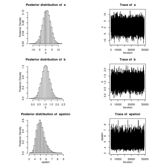
plotMH(mcmc_r)

By default, this will also plot the pair-wise correlation between all parameters.

4) Print posterior Credible Intervals.

BCI(mcmc_r)
#              0.025    0.975
# a       -5.3345970 6.841016
# b        0.4216079 1.690075
# epsilon  3.8863393 6.660037

Tadda! Easy-Peasy.

For a more introductory look at Bayesian modeling, check out the slides and script file from an R workshop I gave at McGill on the subject. There are some additional optional arguments you can pass to Metro_Hastings() which you can read all about in the package manual. You can get the package source from cran, or from my github page.

*notes: MHadaptive is only recommended for relatively low dimensional models. Mixing can be quite slow for higher order models.

Monty Hall by simulation in R

(Almost) every introductory course in probability introduces conditional probability using the famous Monte Hall problem. In a nutshell, the problem is one of deciding on a best strategy in a simple game. In the game, the contestant is asked to select one of three doors. Behind one of the doors is a great prize (free attendance to an R workshop, lets say), and there is a bum prize behind each of the other two doors. The bum prize is usually depicted to be a goat, but I don’t think that would be such a bad prize, so let’s say that behind two of the doors is a bunch of poorly collected data for you to analyse. Once the contestant makes her first selection, the host then opens one of the other two doors to reveal one of the bum prizes.

At this point, the contestant is given the choice to either stay with her original selection, or switch to the other remaining unopened door. What should she do?

If you’re reading this blog, you no doubt gleefully shouted “Switch! Switch! Daddy needs a ticket to that R workshop!”. And you also, no doubt, can prove this to be the best strategy using the logic of probability. You reason that the contestant’s chance of selecting the winning door from the onset was 1/3, giving her a 2/3 probability of being wrong. Once one door with a bum prize has been opened, the contestant is now choosing between two doors. Knowing that there was only a 1/3 chance that original selection was correct, there is now a 2/3 chance that the alternate door is the winner.

As I have mentioned in previous posts, I have found that engaging students to think through logical reasoning problems can be greatly enhanced by appealing to their desire to see it in action. To that end, I whipped up this little script to simulate repeatedly playing the Monte Hall game.


#####################################################
# Simulation of the Monty Hall Problem
# Demonstrates that switching gives you better odds
# than staying with your initial guess
#
# Corey Chivers, 2012
#####################################################

rm(list=ls())
monty<-function(strat='stay',N=1000,print_games=TRUE)
{
 doors<-1:3 #initialize the doors behind one of which is a good prize
 win<-0 #to keep track of number of wins

for(i in 1:N)
 {
 prize<-floor(runif(1,1,4)) #randomize which door has the good prize
 guess<-floor(runif(1,1,4)) #guess a door at random

## Reveal one of the doors you didn't pick which has a bum prize
 if(prize!=guess)
 reveal<-doors[-c(prize,guess)]
 else
 reveal<-sample(doors[-c(prize,guess)],1)

 ## Stay with your initial guess or switch
 if(strat=='switch')
 select<-doors[-c(reveal,guess)]
 if(strat=='stay')
 select<-guess
 if(strat=='random')
 select<-sample(doors[-reveal],1)

## Count up your wins
 if(select==prize)
 {
 win<-win+1
 outcome<-'Winner!'
 }else
 outcome<-'Losser!'

if(print_games)
 cat(paste('Guess: ',guess,
 '\nRevealed: ',reveal,
 '\nSelection: ',select,
 '\nPrize door: ',prize,
 '\n',outcome,'\n\n',sep=''))
 }
 cat(paste('Using the ',strat,' strategy, your win percentage was ',win/N*100,'%\n',sep='')) #Print the win percentage of your strategy
}

Students can then use the function to simulate N games under the strategies ‘stay’, ‘switch’, and ‘random’. Invoking the function using:


monty(strat="stay")
monty(strat="switch")
monty(strat="random")

Hey, look at that – it is better to switch! Feel free to use this in your own class, and let me know if you use it or adapt it in an interesting way!

Edit: Thanks to Ken for pointing out that saying that ‘switching is always better’ is not quite right (you will loose 1/3 of the time, after all), but rather that switching is a rational best strategy, given your state of knowledge.