If you can write the likelihood function for your model, MHadaptive will take care of the rest (ie. all that MCMC business). I wrote this R package to simplify the estimation of posterior distributions of arbitrary models. Here’s how it works:
1) Define your model (ie the likelihood * prior). In this example, lets build a simple linear regression model.
(log)Likelihood:
li_reg<-function(pars,data)
{
a<-pars[1]      #intercept
b<-pars[2]      #slope
sd_e<-pars[3]   #error (residuals)
if(sd_e<=0){return(NaN)}
pred <- a + b * data[,1]
log_likelihood<-sum( dnorm(data[,2],pred,sd_e, log=TRUE) )
prior<- prior_reg(pars)
return(log_likelihood + prior)
}
Prior:
prior_reg<-function(pars)
{
a<-pars[1]          #intercept
b<-pars[2]          #slope
epsilon<-pars[3]    #error

prior_a<-dnorm(a,0,100,log=TRUE)     ## non-informative (flat) priors on all
prior_b<-dnorm(b,0,100,log=TRUE)     ## parameters.
prior_epsilon<-dgamma(epsilon,1,1/100,log=TRUE)

return(prior_a + prior_b + prior_epsilon)
}
Now lets just simulate some data to give it a test run:
x<-runif(30,5,15)
y<-x+rnorm(30,0,5) ##Slope=1, intercept=0, epsilon=5
d<-cbind(x,y)
plot(x,y)
2) The function Metro_Hastings() does all the work. Just pass your model to this function, sit back and let MC Emmcee take it away.
mcmc_r<-Metro_Hastings(li_func=li_reg,pars=c(0,1,1),
par_names=c('a','b','epsilon'),data=d)
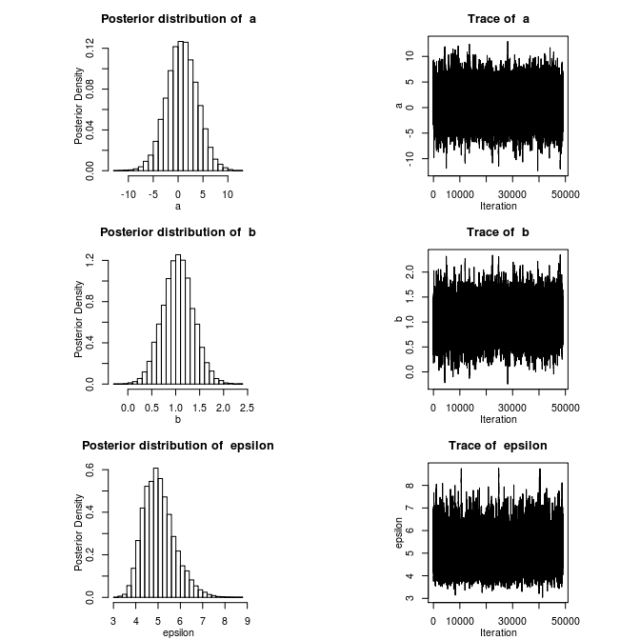
3) You can view the posteriors of all model parameters using plotMH()
plotMH(mcmc_r)
By default, this will also plot the pair-wise correlation between all parameters.
4) Print posterior Credible Intervals.
BCI(mcmc_r)
#              0.025    0.975
# a       -5.3345970 6.841016
# b        0.4216079 1.690075
# epsilon  3.8863393 6.660037
Tadda! Easy-Peasy.
For a more introductory look at Bayesian modeling, check out the slides and script file from an R workshop I gave at McGill on the subject. There are some additional optional arguments you can pass to Metro_Hastings() which you can read all about in the package manual. You can get the package source from cran, or from my github page.
*notes: MHadaptive is only recommended for relatively low dimensional models. Mixing can be quite slow for higher order models.


This is great, and looks very simple to use! To address the slow-mixing issue, we’ve implemented something very similar, whereby the user inputs their density function and 2 algorithms (parallel adaptive MH and a parallel adaptive Wang-Landau algorithm) conduct automatic estimation of the function. You can find the R package here:
http://cran.r-project.org/web/packages/PAWL/index.html
We’ve also written a bit about why automatic Monte Carlo methods are so crucial:
http://arxiv.org/abs/1109.3829
Very cool. I’m checking out PAWL right now. Yours is the first method I have seen which can handle multi-modality in a reliable way. MHadaptive assumes that the target distribution can be adequately approximated by a multivariate normal. Thanks for the note!
Pingback: Visualising the Metropolis-Hastings algorithm « bayesianbiologist
Thanks for making this available with such clear and detailed instructions. Is there any chance you could show how to get an r-squared distribution using MHadaptive? I can see some code here http://www.stat.columbia.edu/~gelman/research/published/rsquared.pdf for BUGS but it would be nice to be able to do it entirely in R. Thanks!
There are two ways I can think of doing this. I’m not 100% sure of either method as in each case it is possible to get R^2 < 0. Both approaches treat R^2 as 1-(residual var of y given model)/(total var of y).
## Using the posterior estimated residual variance (sigma^2):
r_sq<-1-mcmc_r$trace[,3]^2/var(y)
## Using the actual residual variance over the posterior distribution of slope and intercept:
var_res<-sapply(1:length(mcmc_r$trace[,1]),function(i){var(mcmc_r$trace[i,1]+mcmc_r$trace[i,2]*x)})
r_sq<-1-var_res/var(y)
Thanks very much for responding so quickly. The second method does not give r-squared values anything like what I’m getting from lm()… Your first method seems to be right on, thanks again for that.
I’m trying to use Metro_Hasting but i had a proplem can you help me please??
There are several adaptive MH, then can you give me a reference that explain this method with more details?
I try the code by with mi function and always this error occur: Error in optim(pars, li_func, control = list(fnscale = -1), hessian = TRUE, :
function cannot be evaluated at initial parameters
I really don’t know what should I do?please help me.