Chaos. Hectic, seemingly unpredictable, complex dynamics. In a word: fun. I usually stick to the warm and fuzzy world of stochasticity and probability distributions, but this post will be (almost) entirely devoid of randomness. While chaotic dynamics are entirely deterministic, their sensitivity to initial conditions can trick the observer into seeing iid.

In ecology, chaotic dynamics can emerge from a very simple model of population.

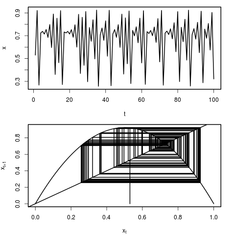
Where the population in time-step t+1 is dependent on the population at time step t, and some intrinsic rate of growth, r. This is known as the logistic (or quadratic) map. For any starting value of x at t₀, the entire evolution of the system can be computed exactly. However, there some values of r for which the system will diverge substantially with even a very slight change in the initial position.

We can see the behaviour of this model by simply plotting the time series of population sizes. Another, and particularly instructive way of visualizing the dynamics, is through the use of a cobweb plot. In this representation, we can see how the population x at time t maps to population x at time t+1 by reflecting through the 1:1 line. Each representation is plotted here:

You can plot realizations of the system using the following R script.

q_map<-function(r=1,x_o=runif(1,0,1),N=100,burn_in=0,...)
{
par(mfrow=c(2,1),mar=c(4,4,1,2),lwd=2)
############# Trace #############
x<-array(dim=N)
x[1]<-x_o
for(i in 2:N)
x[i]<-r*x[i-1]*(1-x[i-1])

plot(x[(burn_in+1):N],type='l',xlab='t',ylab='x',...)
#################################

##########  Quadradic Map ########
x<-seq(from=0,to=1,length.out=100)
x_np1<-array(dim=100)
for(i in 1:length(x))
x_np1[i]<-r*x[i]*(1-x[i])

plot(x,x_np1,type='l',xlab=expression(x[t]),ylab=expression(x[t+1]))
abline(0,1)

start=x_o
vert=FALSE
lines(x=c(start,start),y=c(0,r*start*(1-start)) )
for(i in 1:(2*N))
{
if(vert)
{
lines(x=c(start,start),y=c(start,r*start*(1-start)) )
vert=FALSE
}
else
{
lines(x=c(start,
r*start*(1-start)),
y=c(r*start*(1-start),
r*start*(1-start)) )
vert=TRUE
start=r*start*(1-start)
}
}
#################################
}

To use, simply call the function with any value of r, and a starting position between 0 an 1.

q_map(r=3.84,x_o=0.4)

Fun right?

Now that you’ve tried a few different values of r at a few starting positions, it’s time to look a little closer at what ranges of r values produce chaotic behaviour, which result in stable orbits, and which lead to dampening oscillations toward fixed points. There is a rigorous mathematics behind this kind of analysis of dynamic systems, but we’re just going to do some numerical experimentation using trusty R and a bit of cpu time.

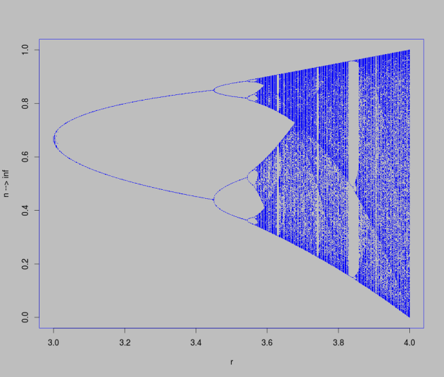
To do this, we’ll need to iterate across a range of r values, and at each one start a dynamical system with a random starting point (told you there would be some randomness in this post). After some large number of time-steps, we’ll record where the system ended up. Plotting the results, we can see a series of period doubling (2,4,8, etc) bifurcations interspersed with regions of chaotic behaviour.

library(parallel)
bifurcation<-function(from=3,to=4,res=500,
x_o=runif(1,0,1),N=500,reps=500,cores=4)
{
r_s<-seq(from=from,to=to,length.out=res)
r<-numeric(res*reps)
for(i in 1:res)
r[((i-1)*reps+1):(i*reps)]<-r_s[i]

x<-array(dim=N)

iterate<-mclapply(1:(res*reps),
mc.cores=cores,
function(k){
x[1]<-runif(1,0,1)
for(i in 2:N)
x[i]<-r[k]*x[i-1]*(1-x[i-1])

return(x[N])
})

plot(r,iterate,pch=15,cex=0.1)

return(cbind(r,iterate))
}

#warning: Even in parallel with 4 cores, this is by no means fast code!
bi<-bifurcation()
png('chaos.png',width=1000,height=850)
par(bg='black',col='green',col.main='green',cex=1)
plot(bi,col='green',xlab='R',ylab='n --> inf',main='',pch=15,cex=0.2)
dev.off()

This plot is known as a bifurcation diagram and is likely a familiar sight.

Hopefully working through the R code and running it yourself will help you interpret cobweb plots, as well as bifurcation diagrams. It is really quite amazing how the simple looking logistic map equation can lead to such interesting behaviour.